Article
Reinforcement learning in robotics:
A survey
The International Journal of
Robotics Research
32(11) 1238–1274
© The Author(s) 2013
Reprints and permissions:
sagepub.co.uk/journalsPermissions.nav
DOI: 10.1177/0278364913495721
ijr.sagepub.com
Jens Kober1,2, J. Andrew Bagnell3 and Jan Peters4,5
Abstract
Reinforcement learning offers to robotics a framework and set of tools for the design of sophisticated and hard-to-engineer
behaviors. Conversely, the challenges of robotic problems provide both inspiration, impact, and validation for develop-
ments in reinforcement learning. The relationship between disciplines has sufficient promise to be likened to that between
physics and mathematics. In this article, we attempt to strengthen the links between the two research communities by
providing a survey of work in reinforcement learning for behavior generation in robots. We highlight both key chal-
lenges in robot reinforcement learning as well as notable successes. We discuss how contributions tamed the complexity
of the domain and study the role of algorithms, representations, and prior knowledge in achieving these successes. As
a result, a particular focus of our paper lies on the choice between model-based and model-free as well as between
value-function-based and policy-search methods. By analyzing a simple problem in some detail we demonstrate how rein-
forcement learning approaches may be profitably applied, and we note throughout open questions and the tremendous
potential for future research.
Keywords
Reinforcement learning, learning control, robot, survey
1. Introduction
A remarkable variety of problems in robotics may be
naturally phrased as problems of reinforcement learning.
Reinforcement learning enables a robot to autonomously
discover an optimal behavior through trial-and-error inter-
actions with its environment. Instead of explicitly detail-
ing the solution to a problem, in reinforcement learning
the designer of a control task provides feedback in terms
of a scalar objective function that measures the one-step
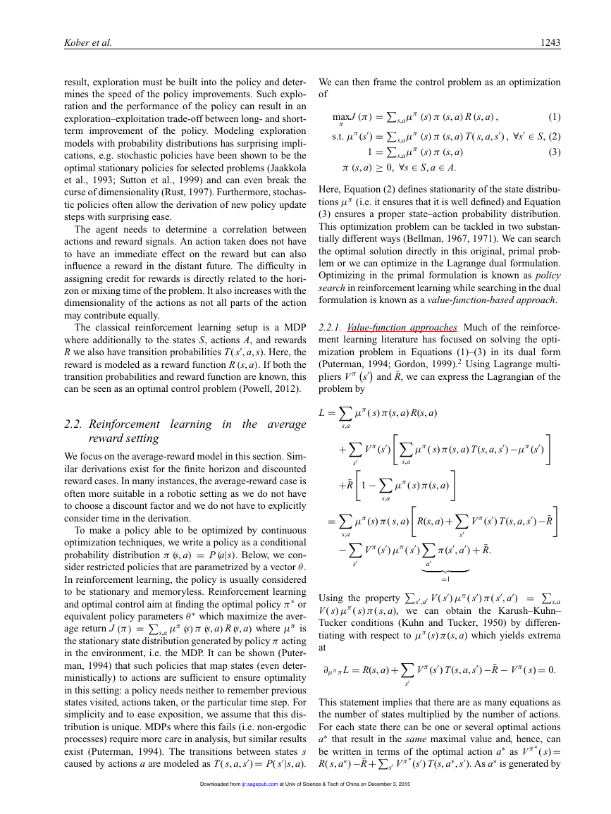
performance of the robot. Figure 1 illustrates the diverse
set of robots that have learned tasks using reinforcement
learning.
Consider, for example, attempting to train a robot to
return a table tennis ball over the net (Muelling et al.,
2012). In this case, the robot might make an observations
of dynamic variables specifying ball position and velocity
and the internal dynamics of the joint position and veloc-
ity. This might in fact capture well the state s of the sys-
tem, providing a complete statistic for predicting future
observations. The actions a available to the robot might
be the torque sent to motors or the desired accelerations
sent to an inverse dynamics control system. A function π
that generates the motor commands (i.e. the actions) based
on the incoming ball and current internal arm observations
(i.e. the state) would be called the policy. A reinforcement
learning problem is to find a policy that optimizes the long-
term sum of rewards R(s, a); a reinforcement learning algo-
rithm is one designed to find such a (near-)optimal policy.
The reward function in this example could be based on the
success of the hits as well as secondary criteria such as
energy consumption.
1.1. Reinforcement
learning in the context of
machine learning
In the problem of reinforcement learning, an agent explores
the space of possible strategies and receives feedback on
1Bielefeld University, CoR-Lab Research Institute for Cognition and
Robotics, Bielefeld, Germany
2Honda Research Institute Europe, Offenbach/Main, Germany
3Carnegie Mellon University, Robotics Institute, Pittsburgh, PA, USA
4Max Planck Institute for Intelligent Systems, Department of Empirical
Inference, Tübingen, Germany
5Technische Universität Darmstadt, FB Informatik, FG Intelligent
Autonomous Systems, Darmstadt, Germany
Corresponding author:
Jens Kober, Bielefeld University, CoR-Lab Research Institute for Cogni-
tion and Robotics, Universitätsstraße 25, 33615 Bielefeld, Germany.
Email: jkober@cor-lab.uni-bielefeld.de
Downloaded from
ijr.sagepub.com
at Univ of Science & Tech of China on December 3, 2015
�
Kober et al.
1239
(a)
(c)
(b)
(d)
Fig. 1. A small sample of robots with behaviors that were rein-
forcement learned. These cover the whole range of aerial vehi-
cles, robotic arms, autonomous vehicles, and humanoid robots.
(a) The OBELIX robot is a wheeled mobile robot that learned
to push boxes (Mahadevan and Connell, 1992) with a value-
function-based approach. (Reprinted with permission from Srid-
har Mahadevan.) (b) A Zebra Zero robot arm learned a peg-in-hole
insertion task (Gullapalli et al., 1994) with a model-free policy
gradient approach. (Reprinted with permission from Rod Gru-
pen.) (c) Carnegie Mellon’s autonomous helicopter leveraged a
model-based policy-search approach to learn a robust flight con-
troller (Bagnell and Schneider, 2001). (d) The Sarcos humanoid
DB learned a pole-balancing task (Schaal, 1996) using forward
models. (Reprinted with permission from Stefan Schaal.)
the outcome of the choices made. From this informa-
tion, a “good”, or ideally optimal, policy (i.e. strategy or
controller) must be deduced.
Reinforcement learning may be understood by contrast-
ing the problem with other areas of study in machine learn-
ing. In supervised learning (Langford and Zadrozny, 2005),
an agent is directly presented a sequence of independent
examples of correct predictions to make in different circum-
stances. In imitation learning, an agent is provided demon-
strations of actions of a good strategy to follow in given
situations (Argall et al., 2009; Schaal, 1999).
To aid in understanding the reinforcement learning prob-
lem and its relation with techniques widely used within
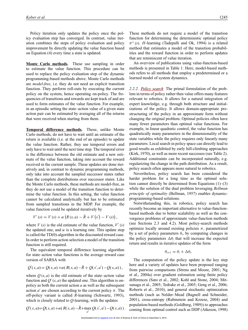
robotics, Figure 2 provides a schematic illustration of two
axes of problem variability: the complexity of sequential
interaction and the complexity of reward structure. This
hierarchy of problems, and the relations between them, is
a complex one, varying in manifold attributes and difficult
to condense to something like a simple linear ordering on
problems. Much recent work in the machine learning com-
munity has focused on understanding the diversity and the
inter-relations between problem classes. The figure should
be understood in this light as providing a crude picture of
the relationship between areas of machine learning research
important for robotics.
Fig. 2. An illustration of the inter-relations between well-studied
learning problems in the literature along axes that attempt to cap-
ture both the information and complexity available in reward sig-
nals and the complexity of sequential interaction between learner
and environment. Each problem subsumes those to the left and
below; reduction techniques provide methods whereby harder
problems (above and right) may be addressed using repeated appli-
cation of algorithms built for simpler problems (Langford and
Zadrozny, 2005).
Each problem subsumes those that are both below and
to the left in the sense that one may always frame the sim-
pler problem in terms of the more complex one; note that
some problems are not linearly ordered. In this sense, rein-
forcement learning subsumes much of the scope of classical
machine learning as well as contextual bandit and imi-
tation learning problems. Reduction algorithms (Langford
and Zadrozny, 2005) are used to convert effective solutions
for one class of problems into effective solutions for others,
and have proven to be a key technique in machine learning.
At lower left, we find the paradigmatic problem of super-
vised learning, which plays a crucial role in applications
as diverse as face detection and spam filtering. In these
problems (including binary classification and regression),
a learner’s goal is to map observations (typically known as
features or covariates) to actions which are usually a dis-
crete set of classes or a real value. These problems possess
no interactive component: the design and analysis of algo-
rithms to address these problems rely on training and testing
instances as independent and identical distributed random
variables. This rules out any notion that a decision made
by the learner will impact future observations: supervised
learning algorithms are built to operate in a world in which
every decision has no effect on the future examples consid-
ered. Further, within supervised learning scenarios, during
a training phase the “correct” or preferred answer is pro-
vided to the learner, so there is no ambiguity about action
choices.
More complex reward structures are also often studied:
one example is known as cost-sensitive learning, where
each training example and each action or prediction is anno-
tated with a cost for making such a prediction. Learning
techniques exist that reduce such problems to the sim-
pler classification problem, and active research directly
addresses such problems as they are crucial in practical
learning applications.
Downloaded from
ijr.sagepub.com
at Univ of Science & Tech of China on December 3, 2015
�
1240
The International Journal of Robotics Research 32(11)
Contextual bandit or associative reinforcement learning
problems begin to address the fundamental problem of
exploration versus exploitation, as information is provided
only about a chosen action and not what might have been.
These find widespread application in problems as diverse as
pharmaceutical drug discovery to ad placement on the web,
and are one of the most active research areas in the field.
Problems of imitation learning and structured prediction
may be seen to vary from supervised learning on the alter-
nate dimension of sequential interaction. Structured pre-
diction, a key technique used within computer vision and
robotics, where many predictions are made in concert by
leveraging inter-relations between them, may be seen as a
simplified variant of imitation learning (Daumé et al., 2009;
Ross et al., 2011a). In imitation learning, we assume that an
expert (for example, a human pilot) that we wish to mimic
provides demonstrations of a task. While “correct answers”
are provided to the learner, complexity arises because any
mistake by the learner modifies the future observations
from what would have been seen had the expert chosen
the controls. Such problems provably lead to compound-
ing errors and violate the basic assumption of independent
examples required for successful supervised learning. In
fact, in sharp contrast with supervised learning problems
where only a single data set needs to be collected, repeated
interaction between learner and teacher appears to both nec-
essary and sufficient (Ross et al., 2011b) to provide perfor-
mance guarantees in both theory and practice in imitation
learning problems.
Reinforcement learning embraces the full complexity of
these problems by requiring both interactive, sequential pre-
diction as in imitation learning as well as complex reward
structures with only “bandit” style feedback on the actions
actually chosen. It is this combination that enables so many
problems of relevance to robotics to be framed in these
terms; it is this same combination that makes the problem
both information-theoretically and computationally hard.
We note here briefly the problem termed “baseline dis-
tribution reinforcement learning”: this is the standard rein-
forcement learning problem with the additional benefit for
the learner that it may draw initial states from a distri-
bution provided by an expert instead of simply an initial
state chosen by the problem. As we describe further in Sec-
tion 5.1, this additional information of which states matter
dramatically affects the complexity of learning.
1.2. Reinforcement
optimal control
learning in the context of
Reinforcement learning is very closely related to the theory
of classical optimal control, as well as dynamic program-
ming, stochastic programming, simulation-optimization,
stochastic search, and optimal stopping (Powell, 2012).
Both reinforcement learning and optimal control address
the problem of finding an optimal policy (often also called
the controller or control policy) that optimizes an objec-
tive function (i.e. the accumulated cost or reward), and
both rely on the notion of a system being described by an
underlying set of states, controls, and a plant or model that
describes transitions between states. However, optimal con-
trol assumes perfect knowledge of the system’s description
in the form of a model (i.e. a function T that describes what
the next state of the robot will be given the current state and
action). For such models, optimal control ensures strong
guarantees which, nevertheless, often break down due to
model and computational approximations. In contrast, rein-
forcement learning operates directly on measured data and
rewards from interaction with the environment. Reinforce-
ment learning research has placed great focus on addressing
cases which are analytically intractable using approxima-
tions and data-driven techniques. One of the most important
approaches to reinforcement learning within robotics cen-
ters on the use of classical optimal control techniques (e.g.
linear-quadratic regulation and differential dynamic pro-
gramming (DDP)) to system models learned via repeated
interaction with the environment (Atkeson, 1998; Bagnell
and Schneider, 2001; Coates et al., 2009). A concise discus-
sion of viewing reinforcement learning as “adaptive optimal
control” is presented by Sutton et al. (1991).
1.3. Reinforcement
learning in the context of
robotics
Robotics as a reinforcement learning domain differs con-
siderably from most well-studied reinforcement learning
benchmark problems. In this article, we highlight
the
challenges faced in tackling these problems. Problems in
robotics are often best represented with high-dimensional,
continuous states and actions (note that the 10–30 dimen-
sional continuous actions common in robot reinforcement
learning are considered large (Powell, 2012)). In robotics,
it is often unrealistic to assume that the true state is com-
pletely observable and noise-free. The learning system will
not be able to know precisely in which state it is and
even vastly different states might look very similar. Thus,
robotics reinforcement learning are often modeled as par-
tially observed, a point we take up in detail in our formal
model description below. The learning system must hence
use filters to estimate the true state. It is often essential
to maintain the information state of the environment that
not only contains the raw observations but also a notion of
uncertainty on its estimates (e.g. both the mean and the vari-
ance of a Kalman filter tracking the ball in the robot table
tennis example).
Experience on a real physical system is tedious to obtain,
expensive and often hard to reproduce. Even getting to the
same initial state is impossible for the robot table tennis sys-
tem. Every single trial run, also called a roll-out, is costly
and, as a result, such applications force us to focus on
difficulties that do not arise as frequently in classical rein-
forcement learning benchmark examples. In order to learn
Downloaded from
ijr.sagepub.com
at Univ of Science & Tech of China on December 3, 2015
�
Kober et al.
1241
within a reasonable time frame, suitable approximations of
state, policy, value function, and/or system dynamics need
to be introduced. However, while real-world experience is
costly, it usually cannot be replaced by learning in simula-
tions alone. In analytical or learned models of the system
even small modeling errors can accumulate to a substan-
tially different behavior, at least for highly dynamic tasks.
Hence, algorithms need to be robust with respect to models
that do not capture all the details of the real system, also
referred to as under-modeling, and to model uncertainty.
Another challenge commonly faced in robot reinforcement
learning is the generation of appropriate reward functions.
Rewards that guide the learning system quickly to success
are needed to cope with the cost of real-world experience.
This problem is called reward shaping (Laud, 2004) and
represents a substantial manual contribution. Specifying
good reward functions in robotics requires a fair amount
of domain knowledge and may often be hard in practice.
Not every reinforcement
learning method is equally
suitable for the robotics domain. In fact, many of the
methods thus far demonstrated on difficult problems have
been model-based (Atkeson et al., 1997; Abbeel et al.,
2007; Deisenroth and Rasmussen, 2011) and robot learn-
ing systems often employ policy-search methods rather than
value-function-based approaches (Gullapalli et al., 1994;
Miyamoto et al., 1996; Bagnell and Schneider, 2001; Kohl
and Stone, 2004; Tedrake et al., 2005; Kober and Peters,
2009; Peters and Schaal, 2008a,b; Deisenroth et al., 2011).
Such design choices stand in contrast to possibly the bulk
of the early research in the machine learning community
(Kaelbling et al., 1996; Sutton and Barto, 1998). We attempt
to give a fairly complete overview on real robot reinforce-
ment learning citing most original papers while grouping
them based on the key insights employed to make the robot
reinforcement learning problem tractable. We isolate key
insights such as choosing an appropriate representation for
a value function or policy, incorporating prior knowledge,
and transfer knowledge from simulations.
This paper surveys a wide variety of tasks where
reinforcement learning has been successfully applied to
robotics. If a task can be phrased as an optimization prob-
lem and exhibits temporal structure, reinforcement learning
can often be profitably applied to both phrase and solve
that problem. The goal of this paper is twofold. On the
one hand, we hope that this paper can provide indications
for the robotics community which type of problems can be
tackled by reinforcement learning and provide pointers to
approaches that are promising. On the other hand, for the
reinforcement learning community, this paper can point out
novel real-world test beds and remarkable opportunities for
research on open questions. We focus mainly on results that
were obtained on physical robots with tasks going beyond
typical reinforcement learning benchmarks.
We concisely present reinforcement learning techniques
in the context of robotics in Section 2. The challenges in
applying reinforcement learning in robotics are discussed
in Section 3. Different approaches to making reinforcement
learning tractable are treated in Sections 4–6. In Section 7,
the example of a ball in a cup is employed to highlight
which of the various approaches discussed in the paper
have been particularly helpful to make such a complex
task tractable. Finally, in Section 8, we summarize the spe-
cific problems and benefits of reinforcement learning in
robotics and provide concluding thoughts on the problems
and promise of reinforcement learning in robotics.
2. A concise introduction to reinforcement
learning
In reinforcement learning, an agent tries to maximize the
accumulated reward over its lifetime. In an episodic setting,
where the task is restarted after each end of an episode, the
objective is to maximize the total reward per episode. If the
task is on-going without a clear beginning and end, either
the average reward over the whole lifetime or a discounted
return (i.e. a weighted average where distant rewards have
less influence) can be optimized. In such reinforcement
learning problems, the agent and its environment may be
modeled being in a state s ∈ S and can perform actions
a ∈ A, each of which may be members of either discrete
or continuous sets and can be multi-dimensional. A state s
contains all relevant information about the current situation
to predict future states (or observables); an example would
be the current position of a robot in a navigation task.1 An
action a is used to control (or change) the state of the sys-
tem. For example, in the navigation task we could have the
actions corresponding to torques applied to the wheels. For
every step, the agent also gets a reward R, which is a scalar
value and assumed to be a function of the state and obser-
vation. (It may equally be modeled as a random variable
that depends on only these variables.) In the navigation task,
a possible reward could be designed based on the energy
costs for taken actions and rewards for reaching targets.
The goal of reinforcement learning is to find a mapping
from states to actions, called policy π, that picks actions
a in given states s maximizing the cumulative expected
reward. The policy π is either deterministic or probabilistic.
The former always uses the exact same action for a given
state in the forma = π( s), the later draws a sample from
a distribution over actions when it encounters a state, i.e.
a ∼ π (s, a) = P (a|s). The reinforcement learning agent
needs to discover the relations between states, actions, and
rewards. Hence, exploration is required which can either be
directly embedded in the policy or performed separately and
only as part of the learning process.
Classical reinforcement learning approaches are based
on the assumption that we have a Markov decision pro-
cess (MDP) consisting of the set of states S, set of actions
A, the rewards R and transition probabilities T that capture
the dynamics of a system. Transition probabilities (or den-
|s, a)
sities in the continuous state case) T( s
describe the effects of the actions on the state. Transition
probabilities generalize the notion of deterministic dynam-
ics to allow for modeling outcomes are uncertain even given
, a, s)= P( s
Downloaded from
ijr.sagepub.com
at Univ of Science & Tech of China on December 3, 2015
�
1242
The International Journal of Robotics Research 32(11)
full state. The Markov property requires that the next state
and the reward only depend on the previous state s and
s
action a (Sutton and Barto, 1998), and not on additional
information about the past states or actions. In a sense, the
Markov property recapitulates the idea of state: a state is a
sufficient statistic for predicting the future, rendering previ-
ous observations irrelevant. In general in robotics, we may
only be able to find some approximate notion of state.
types of
Different
reward functions are commonly
used, including rewards depending only on the current state
R = R( s), rewards depending on the current state and
action R = R( s, a), and rewards including the transitions
R = R( s
, a, s). Most of the theoretical guarantees only
hold if the problem adheres to a Markov structure, how-
ever in practice, many approaches work very well for many
problems that do not fulfill this requirement.
2.1. Goals of reinforcement learning
The goal of reinforcement learning is to discover an optimal
policy π∗
that maps states (or observations) to actions so as
to maximize the expected return J, which corresponds to
the cumulative expected reward. There are different models
of optimal behavior (Kaelbling et al., 1996) which result in
different definitions of the expected return. A finite-horizon
model only attempts to maximize the expected reward for
the horizon H, i.e. the next H (time) steps h
H
Rh
.
h=0
J = E
This setting can also be applied to model problems where it
is known how many steps are remaining.
discount factor γ (with 0 ≤ γ < 1)
Alternatively, future rewards can be discounted by a
J = E
γ hRh
.
∞
h=0
This is the setting most frequently discussed in classical
reinforcement learning texts. The parameter γ affects how
much the future is taken into account and needs to be tuned
manually. As illustrated by Kaelbling et al. (1996), this
parameter often qualitatively changes the form of the opti-
mal solution. Policies designed by optimizing with small
γ are myopic and greedy, and may lead to poor perfor-
mance if we actually care about longer-term rewards. It is
straightforward to show that the optimal control law can
be unstable if the discount factor is too low (e.g. it is not
difficult to show this destabilization even for discounted
linear quadratic regulation problems). Hence, discounted
formulations are frequently inadmissible in robot control.
In the limit when γ approaches 1, the metric approaches
what is known as the average-reward criterion (Bertsekas,
1995),
H
J = lim
H→∞ E
1
H
Rh
.
h=0
This setting has the problem that it cannot distinguish
between policies that initially gain a transient of large
rewards and those that do not. This transient phase, also
called prefix, is dominated by the rewards obtained in the
long run. If a policy accomplishes both an optimal pre-
fix as well as an optimal long-term behavior, it is called
bias optimal (Lewis and Puterman, 2001). An example in
robotics would be the transient phase during the start of a
rhythmic movement, where many policies will accomplish
the same long-term reward but differ substantially in the
transient (e.g. there are many ways of starting the same
gait in dynamic legged locomotion) allowing for room for
improvement in practical application.
In real-world domains, the shortcomings of the dis-
counted formulation are often more critical than those of
the average reward setting as stable behavior is often more
important than a good transient (Peters et al., 2004). We
also often encounter an episodic control task, where the task
runs only for H time steps and then reset (potentially by
human intervention) and started over. This horizon, H, may
be arbitrarily large, as long as the expected reward over the
episode can be guaranteed to converge. As such episodic
tasks are probably the most frequent ones, finite-horizon
models are often the most relevant.
Two natural goals arise for the learner. In the first, we
attempt to find an optimal strategy at the end of a phase of
training or interaction. In the second, the goal is to maxi-
mize the reward over the whole time the robot is interacting
with the world.
In contrast to supervised learning, the learner must first
discover its environment and is not told the optimal action it
needs to take. To gain information about the rewards and the
behavior of the system, the agent needs to explore by con-
sidering previously unused actions or actions it is uncertain
about. It needs to decide whether to play it safe and stick
to well-known actions with (moderately) high rewards or
to dare trying new things in order to discover new strate-
gies with an even higher reward. This problem is commonly
known as the exploration–exploitation trade-off.
In principle,
reinforcement
learning algorithms for
MDPs with performance guarantees are known (Brafman
and Tennenholtz, 2002; Kearns and Singh, 2002; Kakade,
2003) with polynomial scaling in the size of the state and
action spaces, an additive error term, as well as in the hori-
zon length (or a suitable substitute including the discount
factor or “mixing time” (Kearns and Singh, 2002)). How-
ever, state-spaces in robotics problems are often tremen-
dously large as they scale exponentially in the number
of state variables and often are continuous. This chal-
lenge of exponential growth is often referred to as the
curse of dimensionality (Bellman, 1957) (also discussed in
Section 3.1).
Off-policy methods learn independent of the employed
policy, i.e. an explorative strategy that is different from
the desired final policy can be employed during the learn-
ing process. On-policy methods collect sample informa-
tion about the environment using the current policy. As a
Downloaded from
ijr.sagepub.com
at Univ of Science & Tech of China on December 3, 2015
�
Kober et al.
1243
result, exploration must be built into the policy and deter-
mines the speed of the policy improvements. Such explo-
ration and the performance of the policy can result in an
exploration–exploitation trade-off between long- and short-
term improvement of the policy. Modeling exploration
models with probability distributions has surprising impli-
cations, e.g. stochastic policies have been shown to be the
optimal stationary policies for selected problems (Jaakkola
et al., 1993; Sutton et al., 1999) and can even break the
curse of dimensionality (Rust, 1997). Furthermore, stochas-
tic policies often allow the derivation of new policy update
steps with surprising ease.
The agent needs to determine a correlation between
actions and reward signals. An action taken does not have
to have an immediate effect on the reward but can also
influence a reward in the distant future. The difficulty in
assigning credit for rewards is directly related to the hori-
zon or mixing time of the problem. It also increases with the
dimensionality of the actions as not all parts of the action
may contribute equally.
The classical reinforcement learning setup is a MDP
where additionally to the states S, actions A, and rewards
, a, s). Here, the
R we also have transition probabilities T( s
reward is modeled as a reward function R (s, a). If both the
transition probabilities and reward function are known, this
can be seen as an optimal control problem (Powell, 2012).
2.2. Reinforcement
reward setting
learning in the average
We focus on the average-reward model in this section. Sim-
ilar derivations exist for the finite horizon and discounted
reward cases. In many instances, the average-reward case is
often more suitable in a robotic setting as we do not have
to choose a discount factor and we do not have to explicitly
consider time in the derivation.
age return J (π ) =
To make a policy able to be optimized by continuous
optimization techniques, we write a policy as a conditional
probability distribution π (s, a) = P (a|s). Below, we con-
sider restricted policies that are parametrized by a vector θ.
In reinforcement learning, the policy is usually considered
to be stationary and memoryless. Reinforcement learning
and optimal control aim at finding the optimal policy π∗
or
equivalent policy parameters θ∗
which maximize the aver-
μπ (s) π (s, a) R (s, a) where μπ is
the stationary state distribution generated by policy π acting
in the environment, i.e. the MDP. It can be shown (Puter-
man, 1994) that such policies that map states (even deter-
ministically) to actions are sufficient to ensure optimality
in this setting: a policy needs neither to remember previous
states visited, actions taken, or the particular time step. For
simplicity and to ease exposition, we assume that this dis-
tribution is unique. MDPs where this fails (i.e. non-ergodic
processes) require more care in analysis, but similar results
exist (Puterman, 1994). The transitions between states s
|s, a).
caused by actions a are modeled as T( s, a, s
)= P( s
s,a
J (π ) =
) =
1 =
We can then frame the control problem as an optimization
of
max
π
μπ (s) π (s, a) R (s, a) ,
s,a
s.t. μπ (s
s,a
μπ (s) π (s, a) T( s, a, s
μπ (s) π (s, a)
π (s, a) ≥ 0, ∀s ∈ S, a ∈ A.
s,a
) , ∀s
(1)
∈ S, (2)
(3)
Here, Equation (2) defines stationarity of the state distribu-
tions μπ (i.e. it ensures that it is well defined) and Equation
(3) ensures a proper state–action probability distribution.
This optimization problem can be tackled in two substan-
tially different ways (Bellman, 1967, 1971). We can search
the optimal solution directly in this original, primal prob-
lem or we can optimize in the Lagrange dual formulation.
Optimizing in the primal formulation is known as policy
search in reinforcement learning while searching in the dual
formulation is known as a value-function-based approach.
2.2.1. Value-function approaches Much of the reinforce-
ment learning literature has focused on solving the opti-
mization problem in Equations (1)–(3) in its dual form
(Puterman, 1994; Gordon, 1999).2 Using Lagrange multi-
and ¯R, we can express the Lagrangian of the
pliers V π
s
problem by
L =
μπ ( s) π(s, a) T(s, a, s
1 −
μπ ( s) π(s, a) R(s, a)
μπ ( s) π(s, a)
)−μπ (s
V π (s
+
s,a
s,a
s
)
)
+¯R
s,a
−
s
s,a
=
μπ (s) π( s, a)
V π (s
) μπ ( s
s
, a
)
R(s, a)+
π(s
a
)
) T(s, a, s
)−¯R
V π (s
+ ¯R.
=1
) =
, a
s
) π( s
) μπ ( s
s,a V ( s
Using the property
s,a
V ( s) μπ ( s) π( s, a), we can obtain the Karush–Kuhn–
Tucker conditions (Kuhn and Tucker, 1950) by differen-
tiating with respect to μπ (s) π(s, a) which yields extrema
at
∂μπ π L = R(s, a)+
)−¯R − V π ( s)= 0.
) T(s, a, s
V π (s
This statement implies that there are as many equations as
the number of states multiplied by the number of actions.
For each state there can be one or several optimal actions
∗
that result in the same maximal value and, hence, can
a
( s)=
∗
be written in terms of the optimal action a
∗
∗
is generated by
). As a
R( s, a
)−¯R+
∗
) T(s, a
as V π∗
, s
(s
s V π∗
Downloaded from
ijr.sagepub.com
at Univ of Science & Tech of China on December 3, 2015
�
1244
The International Journal of Robotics Research 32(11)
the same optimal policy π∗
multipliers at optimality is
, we know the condition for the
∗
) T(s, a
)
, s
, (4)
∗
V
)−¯R +
∗
R(s, a
( s)= max
a∗
(s) is a shorthand notation for V π∗
(s
V
s
∗
∗
where V
(s). This state-
ment is equivalent to the Bellman principle of optimality
(Bellman, 1957)3 that states “An optimal policy has the
property that whatever the initial state and initial decision
are, the remaining decisions must constitute an optimal pol-
icy with regard to the state resulting from the first decision”.
∗
and, subse-
Thus, we have to perform an optimal action a
quently, follow the optimal policy π∗
in order to achieve
a global optimum. When evaluating Equation (4), we real-
∗ (s) corresponds to the
ize that optimal value function V
long-term additional reward, beyond the average reward ¯R,
∗
gained by starting in state s while taking optimal actions a
(according to the optimal policy π∗
). This principle of opti-
mality has also been crucial in enabling the field of optimal
control (Kirk, 1970).
Hence, we have a dual formulation of the original prob-
lem that serves as condition for optimality. Many traditional
reinforcement learning approaches are based on identifying
(possibly approximate) solutions to this equation, and are
known as value-function methods. Instead of directly learn-
ing a policy, they first approximate the Lagrangian multi-
∗ (s), also called the value function, and use it to
pliers V
reconstruct the optimal policy. The value function V π (s)
is defined equivalently, however instead of always taking
∗
, the action a is picked according to
the optimal action a
a policy π
V π (s)=
π (s, a)
a
R (s, a) − ¯R +
s
V π
s
T
s, a, s
.
Instead of the value function V π (s) many algorithms rely
on the state–action value function Qπ ( s, a) instead, which
has advantages for determining the optimal policy as shown
below. This function is defined as
Qπ (s, a) = R (s, a) − ¯R +
s, a, s
V π
T
s
.
s
In contrast to the value function V π (s), the state–action
value function Qπ (s, a) explicitly contains the informa-
tion about the effects of a particular action. The optimal
state–action value function is
∗ (s, a)= R (s, a) − ¯R +
Q
= R (s, a) − ¯R +
∗
∗
s, a, s
s, a, s
, a
V
s
T
T
s
s
.
max
a Q
s
It can be shown that an optimal, deterministic policy
π∗ (s) can be reconstructed by always picking the action a
∗
a
.
s
s
∗
T
s
V
( s)
s, a, s
s, a, s
∗
in the current state that leads to the state s with the highest
value V
π∗ (s) = arg max
R (s, a) − ¯R +
∗
If the optimal value function V
and the transition
for the following states are known,
probabilities T
determining the optimal policy is straightforward in a set-
ting with discrete actions as an exhaustive search is possi-
ble. For continuous spaces, determining the optimal action
∗
is an optimization problem in itself. If both states and
a
actions are discrete, the value function and the policy may,
in principle, be represented by tables and picking the appro-
priate action is reduced to a look-up. For large or con-
tinuous spaces representing the value function as a table
becomes intractable. Function approximation is employed
to find a lower-dimensional representation that matches the
real value function as closely as possible, as discussed in
∗ (s, a)
Section 2.4. Using the state–action value function Q
instead of the value function V
π∗ (s) = arg max
∗ (s)
∗ (s, a)
Q
,
a
avoids having to calculate the weighted sum over the suc-
cessor states, and hence no knowledge of the transition
function is required.
A wide variety of methods of value-function-based rein-
to estimate
forcement
learning algorithms that attempt
∗ (s) or Q
∗ (s, a) have been developed and can be split
V
mainly into three classes: (i) dynamic programming-based
optimal control approaches such as policy iteration or
value iteration, (ii) rollout-based Monte Carlo methods and
(iii) temporal difference methods such as TD(λ) (Tempo-
ral Difference learning), Q-learning, and SARSA (State–
Action–Reward–State–Action).
Dynamic programming-based methods. These require
, a, s) and the
a model of the transition probabilities T( s
reward function R( s, a) to calculate the value function. The
model does not necessarily need to be predetermined but
can also be learned from data, potentially incrementally.
Such methods are called model-based. Typical methods
include policy iteration and value iteration.
Policy iteration alternates between the two phases of pol-
icy evaluation and policy improvement. The approach is
initialized with an arbitrary policy. Policy evaluation deter-
mines the value function for the current policy. Each state
is visited and its value is updated based on the current
value estimates of its successor states, the associated tran-
sition probabilities, as well as the policy. This procedure
is repeated until the value function converges to a fixed
point, which corresponds to the true value function. Pol-
icy improvement greedily selects the best action in every
state according to the value function as shown above. The
two steps of policy evaluation and policy improvement are
iterated until the policy does not change any longer.
Downloaded from
ijr.sagepub.com
at Univ of Science & Tech of China on December 3, 2015
�
Kober et al.
1245
Policy iteration only updates the policy once the pol-
icy evaluation step has converged. In contrast, value iter-
ation combines the steps of policy evaluation and policy
improvement by directly updating the value function based
on Equation (4) every time a state is updated.
Monte Carlo methods. These use sampling in order
to estimate the value function. This procedure can be
used to replace the policy evaluation step of the dynamic
programming-based methods above. Monte Carlo methods
are model-free, i.e. they do not need an explicit transition
function. They perform roll-outs by executing the current
policy on the system, hence operating on-policy. The fre-
quencies of transitions and rewards are kept track of and are
used to form estimates of the value function. For example,
in an episodic setting the state–action value of a given state
action pair can be estimated by averaging all of the returns
that were received when starting from them.
Temporal difference methods. These, unlike Monte
Carlo methods, do not have to wait until an estimate of the
return is available (i.e. at the end of an episode) to update
the value function. Rather, they use temporal errors and
only have to wait until the next time step. The temporal error
is the difference between the old estimate and a new esti-
mate of the value function, taking into account the reward
received in the current sample. These updates are done iter-
atively and, in contrast to dynamic programming methods,
only take into account the sampled successor states rather
than the complete distributions over successor states. Like
the Monte Carlo methods, these methods are model-free, as
they do not use a model of the transition function to deter-
mine the value function. In this setting, the value function
cannot be calculated analytically but has to be estimated
from sampled transitions in the MDP. For example, the
value function could be updated iteratively by
R (s, a) − ¯R + V
− V (s)
s
(s) = V (s) + α
V
,
(s)
where V (s) is the old estimate of the value function, V
the updated one, and α is a learning rate. This update step
is called the TD(0)-algorithm in the discounted reward case.
In order to perform action selection a model of the transition
function is still required.
Q
, a
The equivalent temporal difference learning algorithm
for state–action value functions is the average reward case
version of SARSA with
( s, a)= Q( s, a)+α( R( s, a)−¯R + Q( s
)−Q( s, a ) ) ,
where Q (s, a) is the old estimate of the state–action value
(s, a) the updated one. This algorithm is on-
function and Q
policy as both the current action a as well as the subsequent
are chosen according to the current policy π. The
action a
off-policy variant is called R-learning (Schwartz, 1993),
which is closely related to Q-learning, with the updates
( s, a)= Q( s, a)+α( R( s, a)−¯R+max
)−Q( s, a ) ) .
, a
Q
a Q( s
These methods do not require a model of the transition
function for determining the deterministic optimal policy
π∗ (s). H-learning (Tadepalli and Ok, 1994) is a related
method that estimates a model of the transition probabil-
ities and the reward function in order to perform updates
that are reminiscent of value iteration.
An overview of publications using value-function-based
methods is presented in Table 1. Here, model-based meth-
ods refers to all methods that employ a predetermined or a
learned model of system dynamics.
2.2.2. Policy search The primal formulation of the prob-
lem in terms of policy rather then value offers many features
relevant to robotics. It allows for a natural integration of
expert knowledge, e.g. through both structure and initial-
izations of the policy. It allows domain-appropriate pre-
structuring of the policy in an approximate form without
changing the original problem. Optimal policies often have
many fewer parameters than optimal value functions. For
example, in linear quadratic control, the value function has
quadratically many parameters in the dimensionality of the
state variables while the policy requires only linearly many
parameters. Local search in policy space can directly lead to
good results as exhibited by early hill-climbing approaches
(Kirk, 1970), as well as more recent successes (see Table 2).
Additional constraints can be incorporated naturally, e.g.
regularizing the change in the path distribution. As a result,
policy search often appears more natural to robotics.
Nevertheless, policy search has been considered the
harder problem for a long time as the optimal solu-
tion cannot directly be determined from Equations (1)–(3)
while the solution of the dual problem leveraging Bellman
principle of optimality (Bellman, 1957) enables dynamic-
programming-based solutions.
Notwithstanding this,
in robotics, policy search has
recently become an important alternative to value-function-
based methods due to better scalability as well as the con-
vergence problems of approximate value-function methods
(see Sections 2.3 and 4.2). Most policy-search methods
optimize locally around existing policies π, parametrized
by a set of policy parameters θi, by computing changes in
the policy parameters �θi that will increase the expected
return and results in iterative updates of the form
θi+1 = θi + �θi.
The computation of the policy update is the key step
here and a variety of updates have been proposed ranging
from pairwise comparisons (Strens and Moore, 2001; Ng
et al., 2004a) over gradient estimation using finite policy
differences (Sato et al., 2002; Kohl and Stone, 2004; Mit-
sunaga et al., 2005; Tedrake et al., 2005; Geng et al., 2006;
Roberts et al., 2010), and general stochastic optimization
methods (such as Nelder–Mead (Bagnell and Schneider,
2001), cross-entropy (Rubinstein and Kroese, 2004) and
population-based methods (Goldberg, 1989)) to approaches
coming from optimal control such as DDP (Atkeson, 1998)
Downloaded from
ijr.sagepub.com
at Univ of Science & Tech of China on December 3, 2015
�




 2023年江西萍乡中考道德与法治真题及答案.doc
 2012年重庆南川中考生物真题及答案.doc
 2013年江西师范大学地理学综合及文艺理论基础考研真题.doc
 2020年四川甘孜小升初语文真题及答案I卷.doc
 2020年注册岩土工程师专业基础考试真题及答案.doc
 2023-2024学年福建省厦门市九年级上学期数学月考试题及答案.doc
 2021-2022学年辽宁省沈阳市大东区九年级上学期语文期末试题及答案.doc
 2022-2023学年北京东城区初三第一学期物理期末试卷及答案.doc
 2018上半年江西教师资格初中地理学科知识与教学能力真题及答案.doc
 2012年河北国家公务员申论考试真题及答案-省级.doc
 2020-2021学年江苏省扬州市江都区邵樊片九年级上学期数学第一次质量检测试题及答案.doc
 2022下半年黑龙江教师资格证中学综合素质真题及答案.doc