c6872_c000.pdf
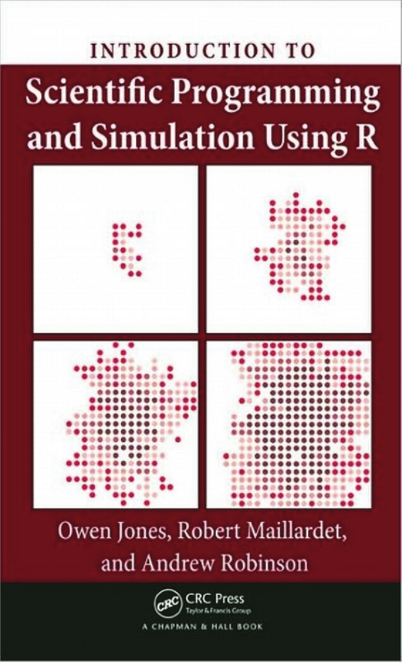
INTRODUCTION TO: Scientific Programming and Simulation Using R
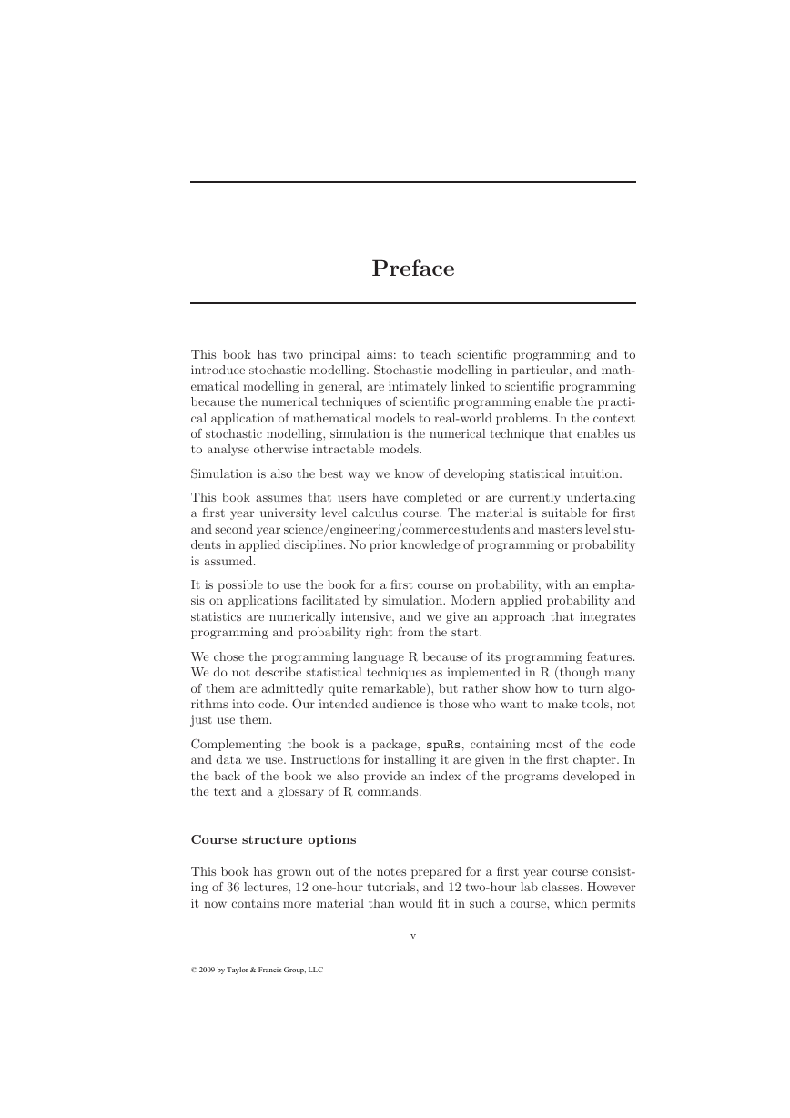
Preface
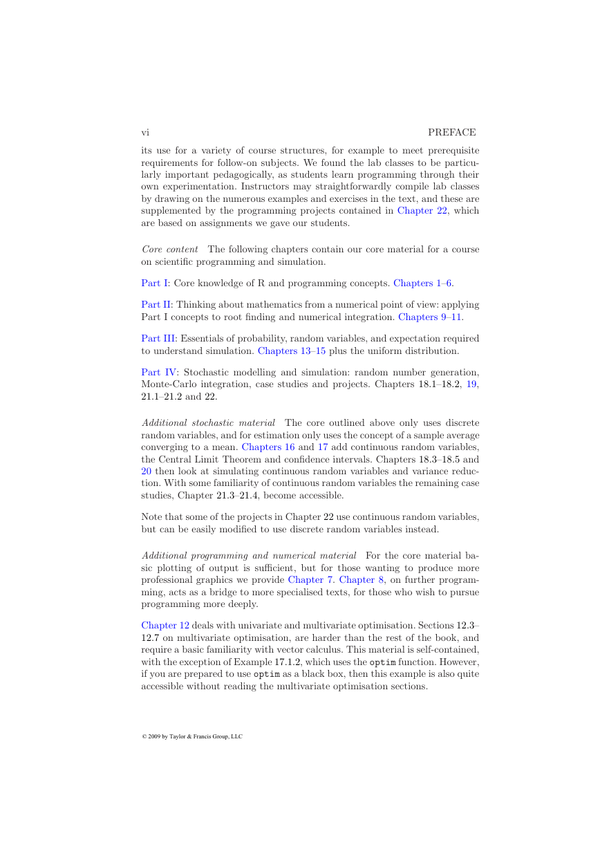
Course structure options
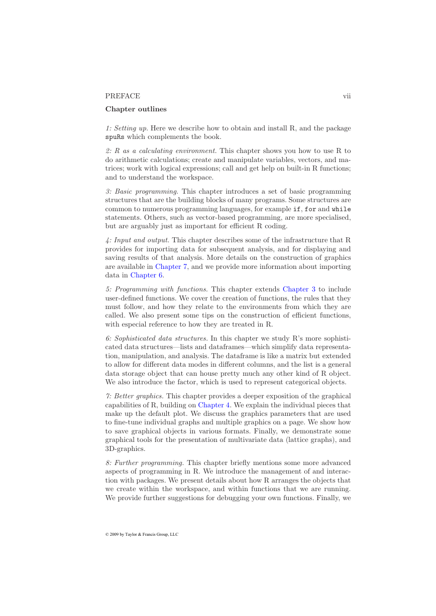
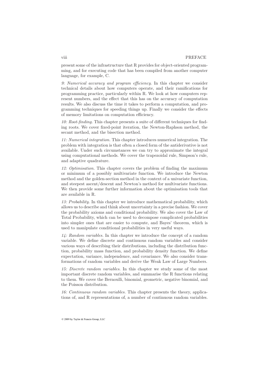
Chapter outlines
Bibliography/further reading
The R language
Scientific programming/numerical techniques
Stochastic modelling and simulation
Caveat computator
Thanks
Contents
Glossary of R commands
Programs and functions developed in the text
c6872_c001.pdf
Table of Contents
PART I: Programming
CHAPTER 1: Setting up
1.1 Installing R
1.2 Starting R
1.3 Working directory
1.4 Writing scripts
1.5 Help
1.6 Supporting material
1.6.1 Installing and loading the package when you have write privileges
1.6.2 Installing and loading the package with limited write privileges
Glossary of R commands
Programs and functions developed in the text
c6872_c002.pdf
Table of Contents
CHAPTER 2: R as a calculating environment
2.1 Arithmetic
2.2 Variables
2.3 Functions
2.4 Vectors
2.4.1 Example: mean and variance
2.4.2 Example: simple numerical integration
2.4.3 Example: exponential limit
2.5 Missing data
2.6 Expressions and assignments
2.7 Logical expressions
2.7.1 Example: rounding error
2.7.2 Sequential && and ||
2.8 Matrices
2.9 The workspace
2.10 Exercises
Glossary of R commands
Programs and functions developed in the text
c6872_c003.pdf
Table of Contents
CHAPTER 3: Basic programming
3.1 Introduction
3.1.1 Example: roots of a quadratic 1 quad1.r
3.2 Branching with if
3.2.1 Example: roots of a quadratic 2 quad2.r
3.3 Looping with for
3.3.1 Example: summing a vector
3.3.2 Example: n factorial 1 nfact1.r
3.3.3 Example: pension value pension.r
3.3.4 Example: redimensioning an array
3.4 Looping with while
3.4.1 Example: Fibonacci numbers fibonacci.r
3.4.2 Example: compound interest compound.r
3.5 Vector-based programming
3.6 Program flow
3.6.1 Pseudo-code
3.7 Basic debugging
3.8 Good programming habits
3.9 Exercises
Glossary of R commands
Programs and functions developed in the text
c6872_c004.pdf
Table of Contents
CHAPTER 4: I/O: Input and Output
4.1 Text
4.2 Input from a file
4.2.1 Example: file input quartiles1.r
4.3 Input from the keyboard
4.3.1 Example: roots of a quadratic 2b quad2b.r
4.4 Output to a file
4.5 Plotting
4.6 Exercises
Glossary of R commands
Programs and functions developed in the text
c6872_c005.pdf
Table of Contents
CHAPTER 5: Programming with functions
5.1 Functions
5.1.1 Example: roots of a quadratic 3 quad3.r
5.1.2 Example: n choose r n_choose_r.r
5.1.3 Example: Winsorised mean wmean.r
5.1.4 Program flow using functions
5.2 Scope and its consequences
5.3 Optional arguments and default values
5.4 Vector-based programming using functions
5.4.1 Example: density of primes primedensity.r
5.5 Recursive programming
5.5.1 Example: n factorial 2 nfact2.r
5.5.2 Example: Sieve of Eratosthenes primesieve.r
5.6 Debugging functions
5.7 Exercises
Glossary of R commands
Programs and functions developed in the text
c6872_c006.pdf
Table of Contents
CHAPTER 6: Sophisticated data structures
6.1 Factors
6.2 Dataframes
6.2.1 Attaching
6.3 Lists
6.3.1 Example: Australian rules football
6.4 The apply family
6.4.1 tapply
6.4.2 Applying functions to lists lapply and sapply
6.4.3 Example: tree growth
6.5 Exercises
Glossary of R commands
Programs and functions developed in the text
c6872_c007.pdf
Table of Contents
CHAPTER 7: Better graphics
7.1 Introduction
7.2 Graphics parameters: par
7.3 Graphical augmentation
7.4 Mathematical typesetting
7.5 Permanence
7.6 Grouped graphs: lattice
7.7 3D-plots
7.8 Exercises
Glossary of R commands
Programs and functions developed in the text
c6872_c008.pdf
Table of Contents
CHAPTER 8: Pointers to further programming techniques
8.1 Packages
8.1.1 Package management
8.1.2 Package construction
8.2 Frames and environments
8.3 Debugging again
8.4 Object-oriented programming: S3
8.4.1 Generic functions
8.4.2 Example: seed dispersal
8.5 Object-oriented programming: S4
8.6 Compiled code
8.6.1 Writing
8.6.2 Compiling
8.6.3 Attaching
8.6.4 Call
8.7 Further reading
8.8 Exercises
Glossary of R commands
Programs and functions developed in the text
c6872_c009.pdf
Table of Contents
PART II: Numerical techniques
CHAPTER 9: Numerical accuracy and program efficiency
9.1 Machine representation of numbers
9.1.1 Integers
9.1.2 Real numbers
9.2 Significant digits
9.2.1 Example: sin(x) − x near 0
9.2.2 Example: range reduction
9.3 Time
9.4 Loops versus vectors
9.4.1 Example: column sums of a matrix
9.5 Memory
9.6 Caveat
9.7 Exercises
Glossary of R commands
Programs and functions developed in the text
c6872_c010.pdf
Table of Contents
CHAPTER 10: Root-finding
10.1 Introduction
10.1.1 Example: loan repayments
10.2 Fixed-point iteration
10.2.1 Example: finding the root of f(x) = log(x) – exp(–x)
10.3 The Newton-Raphson method
10.4 The secant method
10.5 The bisection method
10.6 Exercises
Glossary of R commands
Programs and functions developed in the text
c6872_c011.pdf
Table of Contents
CHAPTER 11: Numerical integration
11.1 Trapezoidal rule
11.2 Simpson’s rule
11.2.1 Example: Phi(z) Phi.r
11.2.2 Example: convergence of Simpson’s rule simpson_test.r
11.2.3 Achieving a set tolerance
11.3 Adaptive quadrature
11.4 Exercises
Glossary of R commands
Programs and functions developed in the text
c6872_c012.pdf
Table of Contents
CHAPTER 12: Optimisation
12.1 Newton’s method for optimisation
12.2 The golden-section method
12.3 Multivariate optimisation
12.4 Steepest ascent
12.4.1 Line search
12.4.2 Example: sin(x2/–y2/4) cos(2x–exp(y))
12.5 Newton’s method in higher dimensions
12.5.1 Example: sin(x2/2–y2/4) cos(2x–exp(y))
12.5.2 On differentiation
12.6 Optimisation in R and the wider world
12.7 A curve fitting example
12.8 Exercises
Glossary of R commands
Programs and functions developed in the text
c6872_c013.pdf
Table of Contents
PART III: Probability and statistics
CHAPTER 13: Probability
13.1 The probability axioms
13.1.1 Counting probability
13.2 Conditional probability
13.2.1 Example: life tables
13.2.2 Example: indigenous deaths in custody
13.3 Independence
13.3.1 Example: disjoint events
13.3.2 Example: the Chevalier de Meré
13.4 The Law of Total Probability
13.5 Bayes’ theorem
13.5.1 Example: prostate cancer screening
13.6 Exercises
Glossary of R commands
Programs and functions developed in the text
c6872_c014.pdf
Table of Contents
CHAPTER 14: Random variables
14.1 Definition and distribution function
14.2 Discrete and continuous random variables
14.3 Empirical cdf’s and histograms
14.3.1 Example: Cavendish’s experiments
14.4 Expectation and finite approximations
14.4.1 Example: numerical calculation of the mean expex.r
14.4.2 Example: truncated normal
14.4.3 Infinite range
14.4.4 Example: gamma function
14.5 Transformations
14.5.1 Transforming a discrete rv
14.5.2 Example: transforming a continuous rv
14.5.3 Expectation of a transformed random variable
14.5.4 Sums of random variables
14.6 Variance and standard deviation
14.7 The Weak Law of Large Numbers
14.7.1 Sample proportion
14.7.2 Sample variance
14.8 Exercises
Glossary of R commands
Programs and functions developed in the text
c6872_c015.pdf
Table of Contents
CHAPTER 15: Discrete random variables
15.1 Discrete random variables in R
15.2 Bernoulli distribution
15.3 Binomial distribution
15.3.1 Example: sampling a manufacturing line
15.4 Geometric distribution
15.4.1 Example: lighting a Barbeque
15.4.2 Example: two-up
15.5 Negative binomial distribution
15.5.1 Example: quality control
15.6 Poisson distribution
15.6.1 Example: the dreaded lurgy
15.6.2 Poisson as a binomial limit
15.7 Exercises
Glossary of R commands
Programs and functions developed in the text
c6872_c016.pdf
Table of Contents
CHAPTER 16: Continuous random variables
16.1 Continuous random variables in R
16.2 Uniform distribution
16.3 Lifetime models: exponential and Weibull
16.3.1 Exponential distribution
16.3.2 Example: radioactive decay
16.3.3 Weibull distribution
16.3.4 Example: time to the next disaster
16.4 The Poisson process and the gamma distribution
16.4.1 A paradox?
16.4.2 Merging and Thinning
16.4.3 Gamma distribution
16.4.4 Example: discrete simulation of a queue
16.5 Sampling distributions: normal, X2, and t
16.5.1 Normal or Gaussian distribution
16.5.2 Example: normal percentage points
16.5.3 The sum of independent normals
16.5.4 X2 distribution
16.5.5 Student’s t distribution
16.6 Exercises
Glossary of R commands
Programs and functions developed in the text
c6872_c017.pdf
Table of Contents
CHAPTER 17: Parameter Estimation
17.1 Point Estimation
17.1.1 Example: Kew rainfall
17.1.2 Example: truncated normal
17.2 The Central Limit Theorem
17.2.1 Proof of the Central Limit Theorem
17.2.2 Normal approximation to the binomial
17.2.3 Continuity correction
17.2.4 Example: insurance risk
17.2.5 Normal approximation to the Poisson
17.2.6 Normal approximation to the negative binomial and gamma
17.3 Confidence intervals
17.3.1 Confidence interval for a proportion
17.3.2 Example: accuracy of an opinion poll
17.3.3 Small sample confidence intervals
17.4 Monte-Carlo confidence intervals
17.4.1 Example: meta-analysis of opinion polls
17.5 Exercises
Glossary of R commands
Programs and functions developed in the text
c6872_c018.pdf
Table of Contents
PART IV: Simulation
CHAPTER 18: Simulation
18.1 Simulating iid uniform samples
18.1.1 Congruential generators
18.1.2 Seeding
18.2 Simulating discrete random variables
18.2.1 Example: binomial
18.2.2 Sequences of independent trials
18.3 Inversion method for continuous rv
18.3.1 Example: uniform distribution
18.3.2 Example: exponential distribution
18.4 Rejection method for continuous rv
18.4.1 Example: triangular density
18.4.2 General rejection method
18.4.3 Efficiency
18.4.4 Example: gamma
18.5 Simulating normals
18.5.1 Central Limit Theorem
18.5.2 Rejection with exponential envelope
18.5.3 Box-Muller algorithm
18.6 Exercises
Glossary of R commands
Programs and functions developed in the text
c6872_c019.pdf
Table of Contents
CHAPTER 19: Monte-Carlo integration
19.1 Hit-and-miss method
19.2 (Improved) Monte-Carlo integration
19.2.1 Lemma
19.2.2 Accuracy in higher dimensions
19.3 Exercises
Glossary of R commands
Programs and functions developed in the text
c6872_c020.pdf
Table of Contents
CHAPTER 20: Variance reduction
20.1 Antithetic sampling
20.1.1 Example: Bu�on’s needle and cross
20.1.2 General antithetic variate technique
20.1.3 Example: improved Monte-Carlo integration
20.1.4 Antithetic pairs through inversion
20.2 Importance sampling
20.2.1 Example: evaluating a simple integral three di�erent ways
20.2.2 Example: standard normal tail probability
20.2.3 Example: standard normal central probability
20.3 Control variates
20.3.1 Example: standard normal central probability
20.4 Exercises
Glossary of R commands
Programs and functions developed in the text
c6872_c021.pdf
Table of Contents
CHAPTER 21: Case studies
21.1 Introduction
21.2 Epidemics
21.2.1 SIR model
21.2.2 Branching processes
21.2.3 Forest fire model
21.3 Inventory
21.3.1 Continuous Review Inventory Model
21.3.2 Simulated inventory level
21.3.3 A two-stage inventory system
21.4 Seed dispersal
21.4.1 Simulating the radial distance R
21.4.2 Object-oriented programming implementation
Glossary of R commands
Programs and functions developed in the text
c6872_c022.pdf
Table of Contents
CHAPTER 22: Student projects
22.1 The level of a dam
22.1.1 Height and volume
22.1.2 Tracking height over time
22.2 Roulette
22.2.1 Simulation
22.2.2 Verification
22.2.3 Variation
22.3 Buffon’s needle and cross
22.3.1 Theoretical analysis
22.3.2 Simulation estimates
22.3.3 Buffon’s cross
22.4 Insurance risk
22.4.1 Simulating X
22.4.2 Simulating Z
22.4.3 Profit taking
22.5 Squash
22.5.1 Status of the game
22.5.2 Simulating a game
22.5.3 Probability of winning
22.5.4 Length of a game
22.6 Stock prices
22.6.1 Simulating S
22.6.2 Estimating ES(t)
22.6.3 Down-and-out call option
Glossary of R commands
Programs and functions developed in the text
c6872_glossary.pdf
Table of Contents
Glossary of R commands
Workspace and help
Objects
Packages
Flow and control and function definition
Mathematical and logical operators and functions
Vectors
Matrices
Dataframes, factors and lists
Input and output
Plotting
Random numbers and probability distributions
Programs and functions developed in the text
c6872_Programs_functions.pdf
Table of Contents
Programs and functions developed in the text
Glossary of R commands


 2023年江西萍乡中考道德与法治真题及答案.doc
 2012年重庆南川中考生物真题及答案.doc
 2013年江西师范大学地理学综合及文艺理论基础考研真题.doc
 2020年四川甘孜小升初语文真题及答案I卷.doc
 2020年注册岩土工程师专业基础考试真题及答案.doc
 2023-2024学年福建省厦门市九年级上学期数学月考试题及答案.doc
 2021-2022学年辽宁省沈阳市大东区九年级上学期语文期末试题及答案.doc
 2022-2023学年北京东城区初三第一学期物理期末试卷及答案.doc
 2018上半年江西教师资格初中地理学科知识与教学能力真题及答案.doc
 2012年河北国家公务员申论考试真题及答案-省级.doc
 2020-2021学年江苏省扬州市江都区邵樊片九年级上学期数学第一次质量检测试题及答案.doc
 2022下半年黑龙江教师资格证中学综合素质真题及答案.doc