8
1
0
2
n
a
J
6
2
]
G
L
.
s
c
[
1
v
0
3
9
8
0
.
1
0
8
1
:
v
i
X
r
a
RECASTING GRADIENT-BASED META-LEARNING AS
HIERARCHICAL BAYES
Erin Grant12, Chelsea Finn12, Sergey Levine12, Trevor Darrell12, Thomas Griffiths13
1 Berkeley AI Research (BAIR), University of California, Berkeley
2 Department of Electrical Engineering & Computer Sciences, University of California, Berkeley
3 Department of Psychology, University of California, Berkeley
{eringrant,cbfinn,svlevine,trevor,tom_griffiths}@berkeley.edu
ABSTRACT
Meta-learning allows an intelligent agent to leverage prior learning episodes as a
basis for quickly improving performance on a novel task. Bayesian hierarchical
modeling provides a theoretical framework for formalizing meta-learning as infer-
ence for a set of parameters that are shared across tasks. Here, we reformulate
the model-agnostic meta-learning algorithm (MAML) of Finn et al. (2017) as a
method for probabilistic inference in a hierarchical Bayesian model. In contrast
to prior methods for meta-learning via hierarchical Bayes, MAML is naturally
applicable to complex function approximators through its use of a scalable gradi-
ent descent procedure for posterior inference. Furthermore, the identification of
MAML as hierarchical Bayes provides a way to understand the algorithm’s op-
eration as a meta-learning procedure, as well as an opportunity to make use of
computational strategies for efficient inference. We use this opportunity to pro-
pose an improvement to the MAML algorithm that makes use of techniques from
approximate inference and curvature estimation.
1
INTRODUCTION
A remarkable aspect of human intelligence is the ability to quickly solve a novel problem and to
be able to do so even in the face of limited experience in a novel domain. Such fast adaptation is
made possible by leveraging prior learning experience in order to improve the efficiency of later
learning. This capacity for meta-learning also has the potential to enable an artificially intelligent
agent to learn more efficiently in situations with little available data or limited computational re-
sources (Schmidhuber, 1987; Bengio et al., 1991; Naik & Mammone, 1992).
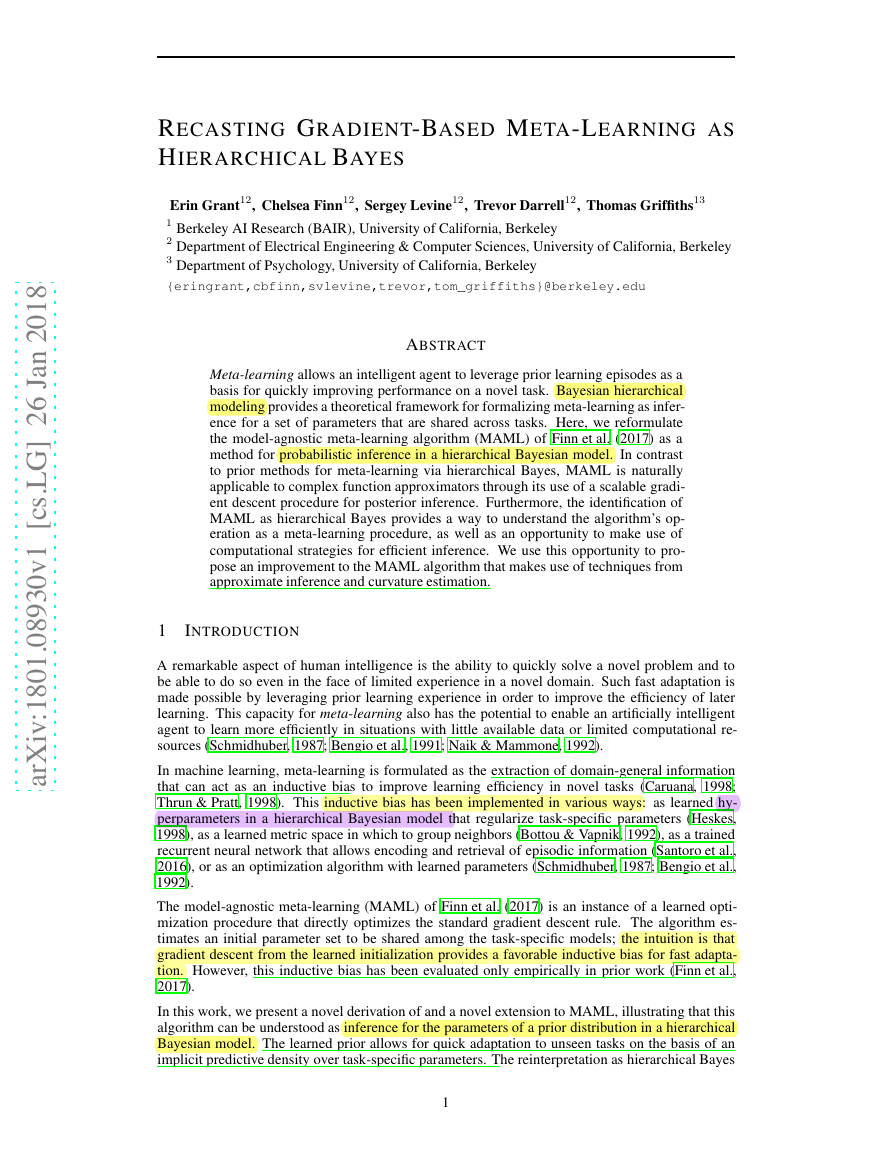
In machine learning, meta-learning is formulated as the extraction of domain-general information
that can act as an inductive bias to improve learning efficiency in novel tasks (Caruana, 1998;
Thrun & Pratt, 1998). This inductive bias has been implemented in various ways: as learned hy-
perparameters in a hierarchical Bayesian model that regularize task-specific parameters (Heskes,
1998), as a learned metric space in which to group neighbors (Bottou & Vapnik, 1992), as a trained
recurrent neural network that allows encoding and retrieval of episodic information (Santoro et al.,
2016), or as an optimization algorithm with learned parameters (Schmidhuber, 1987; Bengio et al.,
1992).
The model-agnostic meta-learning (MAML) of Finn et al. (2017) is an instance of a learned opti-
mization procedure that directly optimizes the standard gradient descent rule. The algorithm es-
timates an initial parameter set to be shared among the task-specific models; the intuition is that
gradient descent from the learned initialization provides a favorable inductive bias for fast adapta-
tion. However, this inductive bias has been evaluated only empirically in prior work (Finn et al.,
2017).
In this work, we present a novel derivation of and a novel extension to MAML, illustrating that this
algorithm can be understood as inference for the parameters of a prior distribution in a hierarchical
Bayesian model. The learned prior allows for quick adaptation to unseen tasks on the basis of an
implicit predictive density over task-specific parameters. The reinterpretation as hierarchical Bayes
1
�
gives a principled statistical motivation for MAML as a meta-learning algorithm, and sheds light
on the reasons for its favorable performance even among methods with significantly more parame-
ters. More importantly, by casting gradient-based meta-learning within a Bayesian framework, we
are able to improve MAML by taking insights from Bayesian posterior estimation as novel aug-
mentations to the gradient-based meta-learning procedure. We experimentally demonstrate that this
enables better performance on a few-shot learning benchmark.
2 META-LEARNING FORMULATION
The goal of a meta-learner is to extract task-general knowledge through the experience of solving
a number of related tasks. By using this learned prior knowledge, the learner has the potential to
quickly adapt to novel tasks even in the face of limited data or limited computation time.
Formally, we consider a dataset D that defines a distribution over a family of tasks T . These tasks
share some common structure such that learning to solve a single task has the potential to aid in
solving another. Each task T defines a distribution over data points x, which we assume in this work
to consist of inputs and either regression targets or classification labels y in a supervised learning
problem (although this assumption can be relaxed to include reinforcement learning problems; e.g.,
see Finn et al., 2017). The objective of the meta-learner is to be able to minimize a task-specific
performance metric associated with any given unseen task from the dataset given even only a small
amount of data from the task; i.e., to be capable of fast adaptation to a novel task.
In the following subsections, we discuss two ways of formulating a solution to the meta-learning
problem: gradient-based hyperparameter optimization and probabilistic inference in a hierarchical
Bayesian model. These approaches were developed orthogonally, but, in Section 3.1, we draw a
novel connection between the two.
2.1 META-LEARNING AS GRADIENT-BASED HYPERPARAMETER OPTIMIZATION
A parametric meta-learner aims to find some shared parameters θ that make it easier to find the right
task-specific parameters φ when faced with a novel task. A variety of meta-learners that employ
gradient methods for task-specific fast adaptation have been proposed (e.g., Andrychowicz et al.,
2016; Li & Malik, 2017a;b; Wichrowska et al., 2017). MAML (Finn et al., 2017) is distinct in that
it provides a gradient-based meta-learning procedure that employs a single additional parameter
(the meta-learning rate) and operates on the same parameter space for both meta-learning and fast
adaptation. These are necessary features for the equivalence we show in Section 3.1.
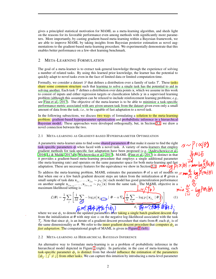
To address the meta-learning problem, MAML estimates the parameters θ of a set of models so
that when one or a few batch gradient descent steps are taken from the initialization at θ given a
small sample of task data xj1 , . . . , xjN
(x) each model has good generalization performance
on another sample xjN +1, . . . , xjN +M ∼ pTj (x) from the same task. The MAML objective in a
maximum likelihood setting is
∼ pTj
L(θ) =
1
J Xj " 1
M Xm
− log p xjN +m | θ − α ∇θ
1
N Xn
− log p xjn | θ
}
{z
φj
#
(1)
|
where we use φj to denote the updated parameters after taking a single batch gradient descent step
from the initialization at θ with step size α on the negative log-likelihood associated with the task
Tj . Note that since φj is an iterate of a gradient descent procedure that starts from θ, each φj is of
the same dimensionality as θ. We refer to the inner gradient descent procedure that computes φj as
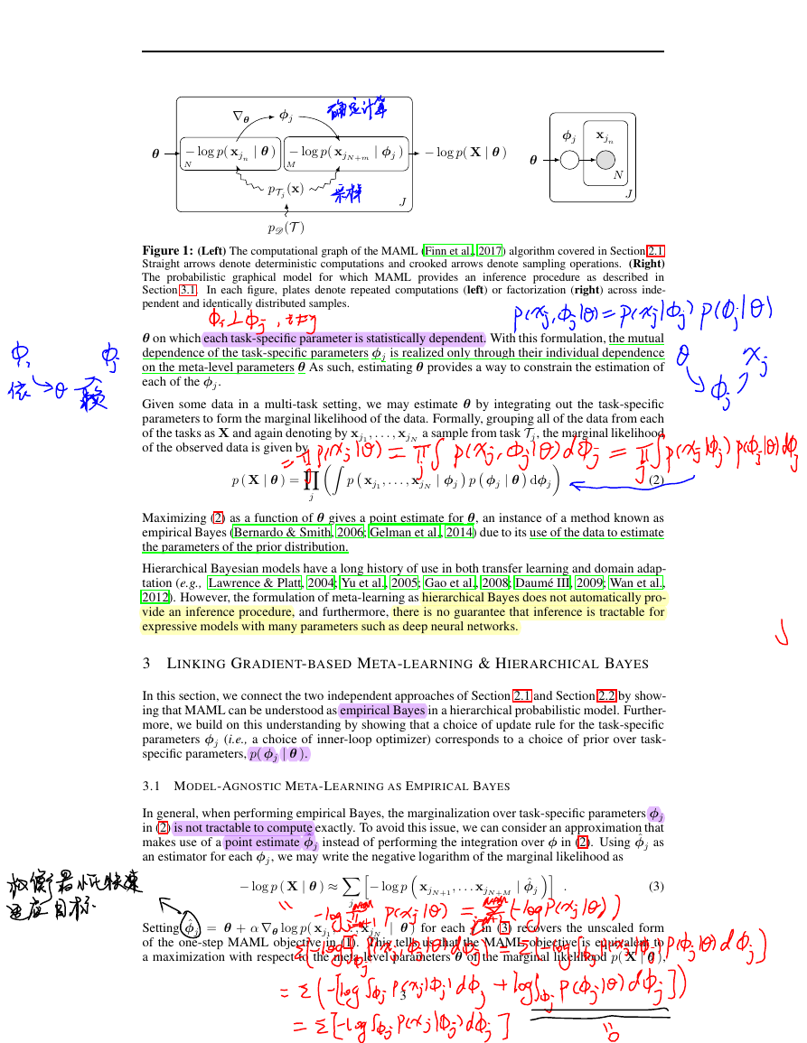
fast adaptation. The computational graph of MAML is given in Figure 1 (left).
2.2 META-LEARNING AS HIERARCHICAL BAYESIAN INFERENCE
An alternative way to formulate meta-learning is as a problem of probabilistic inference in the
hierarchical model depicted in Figure 1 (right). In particular, in the case of meta-learning, each
task-specific parameter φj is distinct from but should influence the estimation of the parameters
′ | j ′ 6= j} from other tasks. We can capture this intuition by introducing a meta-level parameter
{φj
2
�
∇θ
φj
θ
− log p( xjn
N
| θ )
− log p( xjN +m
| φj )
− log p( X | θ )
M
pTj
(x)
pD (T )
J
φj
xjn
θ
N
J
Figure 1: (Left) The computational graph of the MAML (Finn et al., 2017) algorithm covered in Section 2.1.
Straight arrows denote deterministic computations and crooked arrows denote sampling operations. (Right)
The probabilistic graphical model for which MAML provides an inference procedure as described in
In each figure, plates denote repeated computations (left) or factorization (right) across inde-
Section 3.1.
pendent and identically distributed samples.
θ on which each task-specific parameter is statistically dependent. With this formulation, the mutual
dependence of the task-specific parameters φj is realized only through their individual dependence
on the meta-level parameters θ As such, estimating θ provides a way to constrain the estimation of
each of the φj .
Given some data in a multi-task setting, we may estimate θ by integrating out the task-specific
parameters to form the marginal likelihood of the data. Formally, grouping all of the data from each
a sample from task Tj , the marginal likelihood
of the tasks as X and again denoting by xj1 , . . . , xjN
of the observed data is given by
p ( X | θ ) =Yj Z p xj1 , . . . , xjN
| φj p φj | θ dφj .
(2)
Maximizing (2) as a function of θ gives a point estimate for θ, an instance of a method known as
empirical Bayes (Bernardo & Smith, 2006; Gelman et al., 2014) due to its use of the data to estimate
the parameters of the prior distribution.
Hierarchical Bayesian models have a long history of use in both transfer learning and domain adap-
tation (e.g., Lawrence & Platt, 2004; Yu et al., 2005; Gao et al., 2008; Daumé III, 2009; Wan et al.,
2012). However, the formulation of meta-learning as hierarchical Bayes does not automatically pro-
vide an inference procedure, and furthermore, there is no guarantee that inference is tractable for
expressive models with many parameters such as deep neural networks.
3 LINKING GRADIENT-BASED META-LEARNING & HIERARCHICAL BAYES
In this section, we connect the two independent approaches of Section 2.1 and Section 2.2 by show-
ing that MAML can be understood as empirical Bayes in a hierarchical probabilistic model. Further-
more, we build on this understanding by showing that a choice of update rule for the task-specific
parameters φj (i.e., a choice of inner-loop optimizer) corresponds to a choice of prior over task-
specific parameters, p( φj | θ ).
3.1 MODEL-AGNOSTIC META-LEARNING AS EMPIRICAL BAYES
In general, when performing empirical Bayes, the marginalization over task-specific parameters φj
in (2) is not tractable to compute exactly. To avoid this issue, we can consider an approximation that
makes use of a point estimate ˆφj instead of performing the integration over φ in (2). Using ˆφj as
an estimator for each φj , we may write the negative logarithm of the marginal likelihood as
− log p ( X | θ ) ≈Xj h− log p xjN +1, . . . xjN +M
| ˆφji .
(3)
Setting ˆφj = θ + α ∇θ log p( xj1 , . . . , xjN | θ ) for each j in (3) recovers the unscaled form
of the one-step MAML objective in (1). This tells us that the MAML objective is equivalent to
a maximization with respect to the meta-level parameters θ of the marginal likelihood p( X | θ ),
3
�
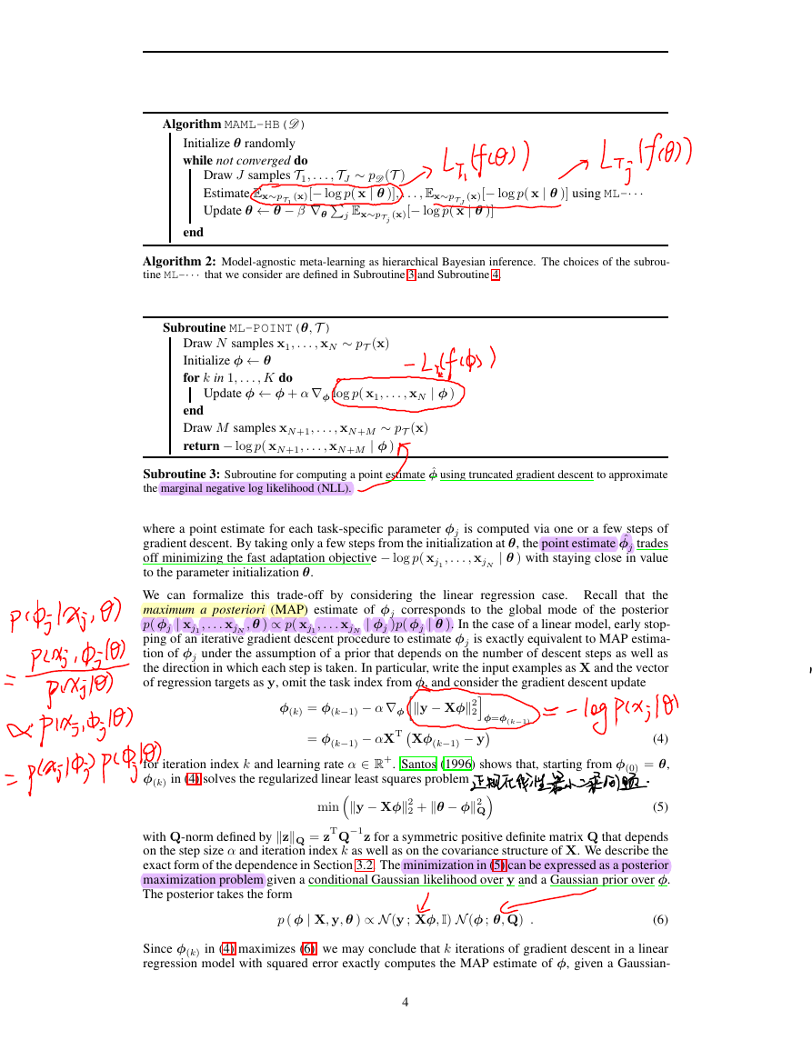
Algorithm MAML-HB(D )
Initialize θ randomly
while not converged do
Draw J samples T1, . . . , TJ ∼ pD (T )
Estimate E
(x)[− log p( x | θ )], . . . , E
x∼pT1
x∼pT
J
E
x∼pT
j
(x)[− log p( x | θ )]
Update θ ← θ − β ∇θPj
end
(x)[− log p( x | θ )] using ML-· · ·
Algorithm 2: Model-agnostic meta-learning as hierarchical Bayesian inference. The choices of the subrou-
tine ML-· · · that we consider are defined in Subroutine 3 and Subroutine 4.
Subroutine ML-POINT(θ, T )
Draw N samples x1, . . . , xN ∼ pT (x)
Initialize φ ← θ
for k in 1, . . . , K do
Update φ ← φ + α ∇φ log p( x1, . . . , xN | φ )
end
Draw M samples xN +1, . . . , xN +M ∼ pT (x)
return − log p( xN +1, . . . , xN +M | φ )
Subroutine 3: Subroutine for computing a point estimate ˆφ using truncated gradient descent to approximate
the marginal negative log likelihood (NLL).
where a point estimate for each task-specific parameter φj is computed via one or a few steps of
gradient descent. By taking only a few steps from the initialization at θ, the point estimate ˆφj trades
off minimizing the fast adaptation objective − log p( xj1 , . . . , xjN
| θ ) with staying close in value
to the parameter initialization θ.
We can formalize this trade-off by considering the linear regression case. Recall that the
maximum a posteriori (MAP) estimate of φj corresponds to the global mode of the posterior
p( φj | xj1 , . . . xjN
| φj )p( φj | θ ). In the case of a linear model, early stop-
ping of an iterative gradient descent procedure to estimate φj is exactly equivalent to MAP estima-
tion of φj under the assumption of a prior that depends on the number of descent steps as well as
the direction in which each step is taken. In particular, write the input examples as X and the vector
of regression targets as y, omit the task index from φ, and consider the gradient descent update
, θ ) ∝ p( xj1 , . . . xjN
(4)
for iteration index k and learning rate α ∈ R+. Santos (1996) shows that, starting from φ(0) = θ,
φ(k) in (4) solves the regularized linear least squares problem
2iφ=φ(k−1)
φ(k) = φ(k−1) − α ∇φhky − Xφk2
= φ(k−1) − αXTXφ(k−1) − y
Q
minky − Xφk2
2 + kθ − φk2
(5)
with Q-norm defined by kzkQ = zTQ
−1z for a symmetric positive definite matrix Q that depends
on the step size α and iteration index k as well as on the covariance structure of X. We describe the
exact form of the dependence in Section 3.2. The minimization in (5) can be expressed as a posterior
maximization problem given a conditional Gaussian likelihood over y and a Gaussian prior over φ.
The posterior takes the form
p ( φ | X, y, θ ) ∝ N (y ; Xφ, I) N (φ ; θ, Q) .
(6)
Since φ(k) in (4) maximizes (6), we may conclude that k iterations of gradient descent in a linear
regression model with squared error exactly computes the MAP estimate of φ, given a Gaussian-
4
�
noised observation model and a Gaussian prior over φ with parameters µ0 = θ and Σ0 = Q. There-
fore, in the case of linear regression with squared error, MAML is exactly empirical Bayes using the
MAP estimate as the point estimate of φ.
In the nonlinear case, MAML is again equivalent to an empirical Bayes procedure to maximize the
marginal likelihood that uses a point estimate for φ computed by one or a few steps of gradient
descent. However, this point estimate is not necessarily the global mode of a posterior. We can
instead understand the point estimate given by truncated gradient descent as the value of the mode of
an implicit posterior over φ resulting from an empirical loss interpreted as a negative log-likelihood,
and regularization penalties and the early stopping procedure jointly acting as priors (for similar
interpretations, see Sjöberg & Ljung, 1995; Bishop, 1995; Duvenaud et al., 2016).
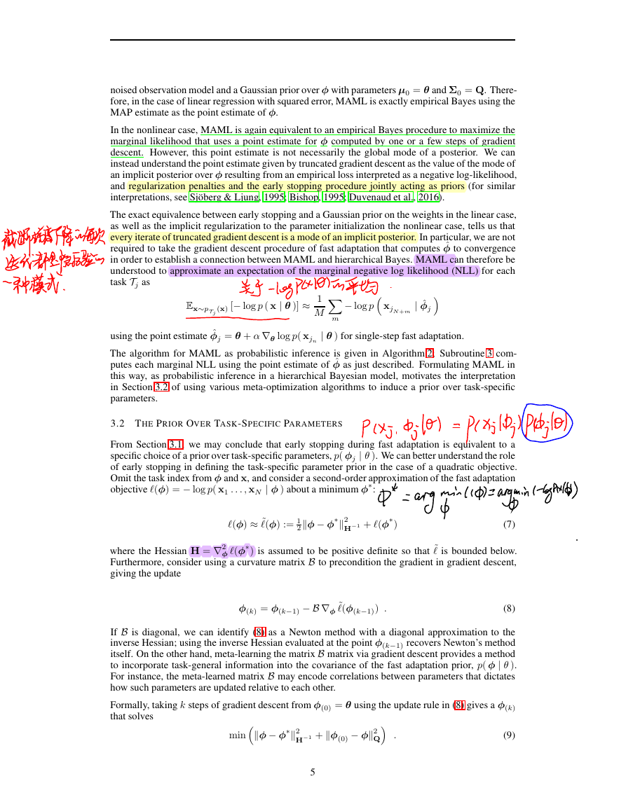
The exact equivalence between early stopping and a Gaussian prior on the weights in the linear case,
as well as the implicit regularization to the parameter initialization the nonlinear case, tells us that
every iterate of truncated gradient descent is a mode of an implicit posterior. In particular, we are not
required to take the gradient descent procedure of fast adaptation that computes ˆφ to convergence
in order to establish a connection between MAML and hierarchical Bayes. MAML can therefore be
understood to approximate an expectation of the marginal negative log likelihood (NLL) for each
task Tj as
E
x∼pT
j
(x) [− log p ( x | θ )] ≈
1
M Xm
− log p xjN +m | ˆφj
using the point estimate ˆφj = θ + α ∇θ log p( xjn | θ ) for single-step fast adaptation.
The algorithm for MAML as probabilistic inference is given in Algorithm 2; Subroutine 3 com-
putes each marginal NLL using the point estimate of ˆφ as just described. Formulating MAML in
this way, as probabilistic inference in a hierarchical Bayesian model, motivates the interpretation
in Section 3.2 of using various meta-optimization algorithms to induce a prior over task-specific
parameters.
3.2 THE PRIOR OVER TASK-SPECIFIC PARAMETERS
From Section 3.1, we may conclude that early stopping during fast adaptation is equivalent to a
specific choice of a prior over task-specific parameters, p( φj | θ ). We can better understand the role
of early stopping in defining the task-specific parameter prior in the case of a quadratic objective.
Omit the task index from φ and x, and consider a second-order approximation of the fast adaptation
objective ℓ(φ) = − log p( x1 . . . , xN | φ ) about a minimum φ
:
∗
ℓ(φ) ≈ ˜ℓ(φ) := 1
2 kφ − φ
∗k2
H
−1 + ℓ(φ
∗)
(7)
where the Hessian H = ∇2
∗) is assumed to be positive definite so that ˜ℓ is bounded below.
Furthermore, consider using a curvature matrix B to precondition the gradient in gradient descent,
giving the update
φ ℓ(φ
φ(k) = φ(k−1) − B ∇φ
˜ℓ(φ(k−1)) .
(8)
If B is diagonal, we can identify (8) as a Newton method with a diagonal approximation to the
inverse Hessian; using the inverse Hessian evaluated at the point φ(k−1) recovers Newton’s method
itself. On the other hand, meta-learning the matrix B matrix via gradient descent provides a method
to incorporate task-general information into the covariance of the fast adaptation prior, p( φ | θ ).
For instance, the meta-learned matrix B may encode correlations between parameters that dictates
how such parameters are updated relative to each other.
Formally, taking k steps of gradient descent from φ(0) = θ using the update rule in (8) gives a φ(k)
that solves
minkφ − φ
∗k2
H
−1 + kφ(0) − φk2
Q .
5
(9)
�
The minimization in (9) corresponds to taking a Gaussian prior p( φ | θ ) with mean θ and co-
−1((I − BΛ)−k − I)OT (Santos, 1996) where B is a diagonal matrix
variance Q for Q = OΛ
that results from a simultaneous diagonalization of H and B as OTHO = diag(λ1, . . . , λn) = Λ
and OTB−1O = diag(b1, . . . , bn) = B with bi, λi ≥ 0 for i = 1, . . . , n (Theorem 8.7.1 in
If the true objective is indeed quadratic, then, assuming the data is
Golub & Van Loan, 1983).
centered, H is the unscaled covariance matrix of features, XTX.
4
IMPROVING MODEL-AGNOSTIC META-LEARNING
Identifying MAML as a method for probabilistic inference in a hierarchical model allows us to de-
velop novel improvements to the algorithm. In Section 4.1, we consider an approach from Bayesian
parameter estimation to improve the MAML algorithm, and in Section 4.2, we discuss how to make
this procedure computationally tractable for high-dimensional models.
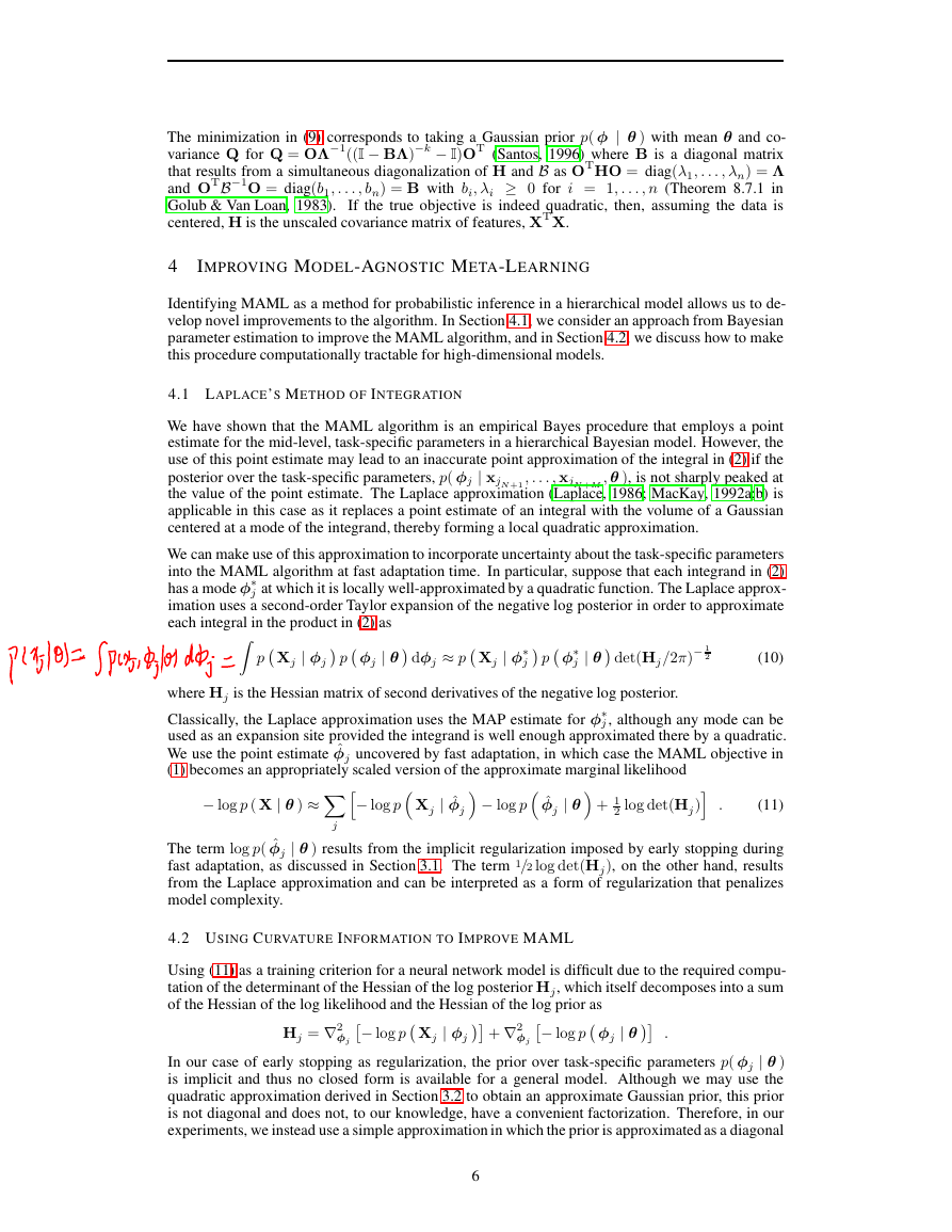
4.1 LAPLACE’S METHOD OF INTEGRATION
We have shown that the MAML algorithm is an empirical Bayes procedure that employs a point
estimate for the mid-level, task-specific parameters in a hierarchical Bayesian model. However, the
use of this point estimate may lead to an inaccurate point approximation of the integral in (2) if the
posterior over the task-specific parameters, p( φj | xjN +1, . . . , xjN +M , θ ), is not sharply peaked at
the value of the point estimate. The Laplace approximation (Laplace, 1986; MacKay, 1992a;b) is
applicable in this case as it replaces a point estimate of an integral with the volume of a Gaussian
centered at a mode of the integrand, thereby forming a local quadratic approximation.
We can make use of this approximation to incorporate uncertainty about the task-specific parameters
into the MAML algorithm at fast adaptation time. In particular, suppose that each integrand in (2)
∗
has a mode φ
j at which it is locally well-approximated by a quadratic function. The Laplace approx-
imation uses a second-order Taylor expansion of the negative log posterior in order to approximate
each integral in the product in (2) as
Z p Xj | φj p φj | θ dφj ≈ p Xj | φ
∗
j p φ
∗
j | θ det(Hj/2π)− 1
2
where Hj is the Hessian matrix of second derivatives of the negative log posterior.
(10)
∗
Classically, the Laplace approximation uses the MAP estimate for φ
j , although any mode can be
used as an expansion site provided the integrand is well enough approximated there by a quadratic.
We use the point estimate ˆφj uncovered by fast adaptation, in which case the MAML objective in
(1) becomes an appropriately scaled version of the approximate marginal likelihood
− log p ( X | θ ) ≈Xj h− log p Xj | ˆφj − log p ˆφj | θ + 1
2 log det(Hj)i .
(11)
The term log p( ˆφj | θ ) results from the implicit regularization imposed by early stopping during
fast adaptation, as discussed in Section 3.1. The term 1/2 log det(Hj), on the other hand, results
from the Laplace approximation and can be interpreted as a form of regularization that penalizes
model complexity.
4.2 USING CURVATURE INFORMATION TO IMPROVE MAML
Using (11) as a training criterion for a neural network model is difficult due to the required compu-
tation of the determinant of the Hessian of the log posterior Hj , which itself decomposes into a sum
of the Hessian of the log likelihood and the Hessian of the log prior as
Hj = ∇2
φj− log p Xj | φj + ∇2
φj− log p φj | θ .
In our case of early stopping as regularization, the prior over task-specific parameters p( φj | θ )
is implicit and thus no closed form is available for a general model. Although we may use the
quadratic approximation derived in Section 3.2 to obtain an approximate Gaussian prior, this prior
is not diagonal and does not, to our knowledge, have a convenient factorization. Therefore, in our
experiments, we instead use a simple approximation in which the prior is approximated as a diagonal
6
�
Subroutine ML-LAPLACE(θ, T )
Draw N samples x1, . . . , xN ∼ pT (x)
Initialize φ ← θ
for k in 1, . . . , K do
Update φ ← φ + α ∇φ log p( x1, . . . , xN | φ )
end
Draw M samples xN +1, . . . , xN +M ∼ pT (x)
Estimate quadratic curvature ˆH
return − log p( xN +1, . . . , xN +M | φ ) + η log det( ˆH)
Subroutine 4: Subroutine for computing a Laplace approximation of the marginal likelihood.
Gaussian with precision τ . We keep τ fixed, although this parameter may be cross-validated for
improved performance.
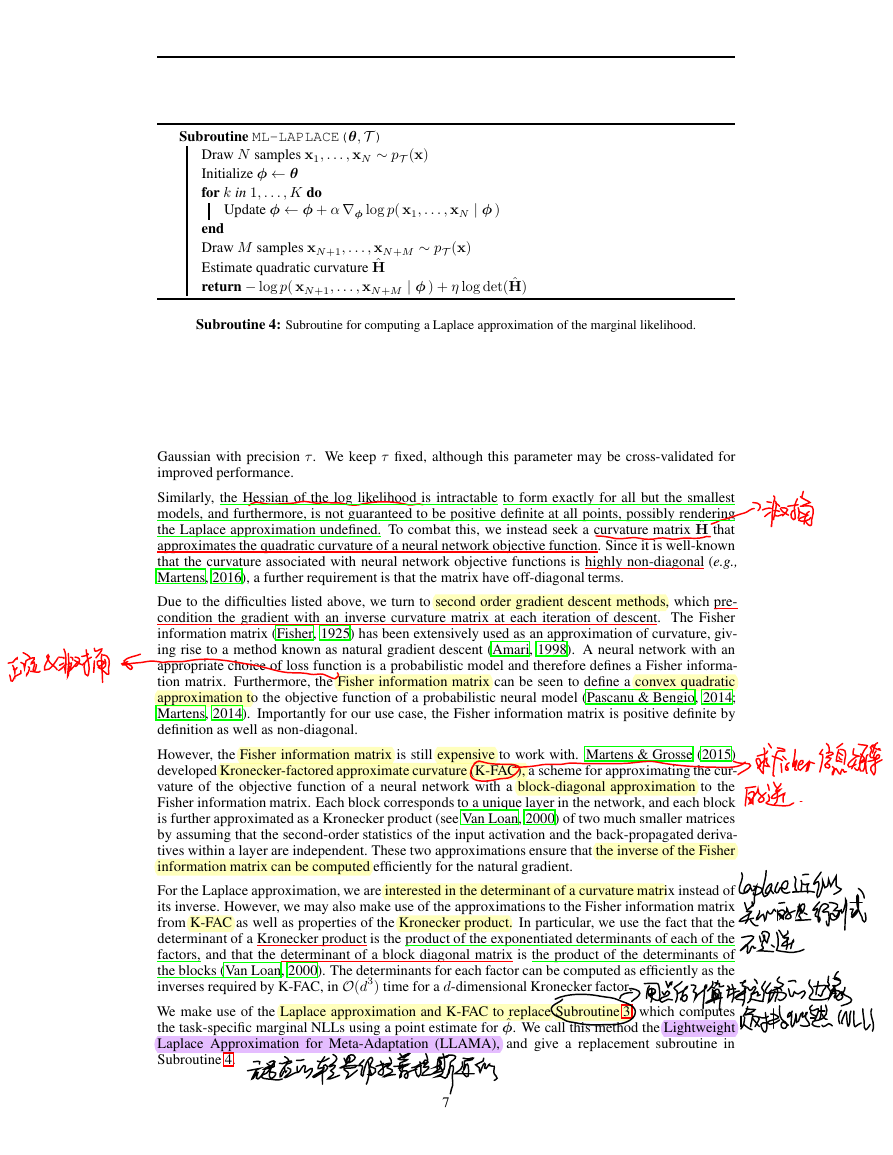
Similarly, the Hessian of the log likelihood is intractable to form exactly for all but the smallest
models, and furthermore, is not guaranteed to be positive definite at all points, possibly rendering
the Laplace approximation undefined. To combat this, we instead seek a curvature matrix ˆH that
approximates the quadratic curvature of a neural network objective function. Since it is well-known
that the curvature associated with neural network objective functions is highly non-diagonal (e.g.,
Martens, 2016), a further requirement is that the matrix have off-diagonal terms.
Due to the difficulties listed above, we turn to second order gradient descent methods, which pre-
condition the gradient with an inverse curvature matrix at each iteration of descent. The Fisher
information matrix (Fisher, 1925) has been extensively used as an approximation of curvature, giv-
ing rise to a method known as natural gradient descent (Amari, 1998). A neural network with an
appropriate choice of loss function is a probabilistic model and therefore defines a Fisher informa-
tion matrix. Furthermore, the Fisher information matrix can be seen to define a convex quadratic
approximation to the objective function of a probabilistic neural model (Pascanu & Bengio, 2014;
Martens, 2014). Importantly for our use case, the Fisher information matrix is positive definite by
definition as well as non-diagonal.
However, the Fisher information matrix is still expensive to work with. Martens & Grosse (2015)
developed Kronecker-factored approximate curvature (K-FAC), a scheme for approximating the cur-
vature of the objective function of a neural network with a block-diagonal approximation to the
Fisher information matrix. Each block corresponds to a unique layer in the network, and each block
is further approximated as a Kronecker product (see Van Loan, 2000) of two much smaller matrices
by assuming that the second-order statistics of the input activation and the back-propagated deriva-
tives within a layer are independent. These two approximations ensure that the inverse of the Fisher
information matrix can be computed efficiently for the natural gradient.
For the Laplace approximation, we are interested in the determinant of a curvature matrix instead of
its inverse. However, we may also make use of the approximations to the Fisher information matrix
from K-FAC as well as properties of the Kronecker product. In particular, we use the fact that the
determinant of a Kronecker product is the product of the exponentiated determinants of each of the
factors, and that the determinant of a block diagonal matrix is the product of the determinants of
the blocks (Van Loan, 2000). The determinants for each factor can be computed as efficiently as the
inverses required by K-FAC, in O(d3) time for a d-dimensional Kronecker factor.
We make use of the Laplace approximation and K-FAC to replace Subroutine 3, which computes
the task-specific marginal NLLs using a point estimate for ˆφ. We call this method the Lightweight
Laplace Approximation for Meta-Adaptation (LLAMA), and give a replacement subroutine in
Subroutine 4.
7
�
5
0
−5
5
0
−5
ground truth func-
tion
few-shot
examples
training
model prediction
sample
model
from the
−10
−5
0
5
10
−10
−5
0
5
10
MAML
MAML with uncertainty
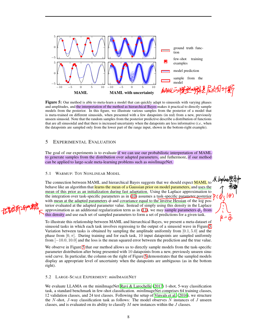
Figure 5: Our method is able to meta-learn a model that can quickly adapt to sinusoids with varying phases
and amplitudes, and the interpretation of the method as hierarchical Bayes makes it practical to directly sample
models from the posterior.
In this figure, we illustrate various samples from the posterior of a model that
is meta-trained on different sinusoids, when presented with a few datapoints (in red) from a new, previously
unseen sinusoid. Note that the random samples from the posterior predictive describe a distribution of functions
that are all sinusoidal and that there is increased uncertainty when the datapoints are less informative (i.e., when
the datapoints are sampled only from the lower part of the range input, shown in the bottom-right example).
5 EXPERIMENTAL EVALUATION
The goal of our experiments is to evaluate if we can use our probabilistic interpretation of MAML
to generate samples from the distribution over adapted parameters, and futhermore, if our method
can be applied to large-scale meta-learning problems such as miniImageNet.
5.1 WARMUP: TOY NONLINEAR MODEL
The connection between MAML and hierarchical Bayes suggests that we should expect MAML to
behave like an algorithm that learns the mean of a Gaussian prior on model parameters, and uses the
mean of this prior as an initialization during fast adaptation. Using the Laplace approximation to
the integration over task-specific parameters as in (10) assumes a task-specific parameter posterior
with mean at the adapted parameters ˆφ and covariance equal to the inverse Hessian of the log pos-
terior evaluated at the adapted parameter value. Instead of simply using this density in the Laplace
approximation as an additional regularization term as in (11), we may sample parameters φj from
this density and use each set of sampled parameters to form a set of predictions for a given task.
To illustrate this relationship between MAML and hierarchical Bayes, we present a meta-dataset of
sinusoid tasks in which each task involves regressing to the output of a sinusoid wave in Figure 5.
Variation between tasks is obtained by sampling the amplitude uniformly from [0.1, 5.0] and the
phase from [0, π]. During training and for each task, 10 input datapoints are sampled uniformly
from [−10.0, 10.0] and the loss is the mean squared error between the prediction and the true value.
We observe in Figure 5 that our method allows us to directly sample models from the task-specific
parameter distribution after being presented with 10 datapoints from a new, previously unseen sinu-
soid curve. In particular, the column on the right of Figure 5 demonstrates that the sampled models
display an appropriate level of uncertainty when the datapoints are ambiguous (as in the bottom
right).
5.2 LARGE-SCALE EXPERIMENT: miniIMAGENET
We evaluate LLAMA on the miniImageNet Ravi & Larochelle (2017) 1-shot, 5-way classification
task, a standard benchmark in few-shot classification. miniImageNet comprises 64 training classes,
12 validation classes, and 24 test classes. Following the setup of Vinyals et al. (2016), we structure
the N -shot, J -way classification task as follows: The model observes N instances of J unseen
classes, and is evaluated on its ability to classify M new instances within the J classes.
8
�


 2023年江西萍乡中考道德与法治真题及答案.doc
 2012年重庆南川中考生物真题及答案.doc
 2013年江西师范大学地理学综合及文艺理论基础考研真题.doc
 2020年四川甘孜小升初语文真题及答案I卷.doc
 2020年注册岩土工程师专业基础考试真题及答案.doc
 2023-2024学年福建省厦门市九年级上学期数学月考试题及答案.doc
 2021-2022学年辽宁省沈阳市大东区九年级上学期语文期末试题及答案.doc
 2022-2023学年北京东城区初三第一学期物理期末试卷及答案.doc
 2018上半年江西教师资格初中地理学科知识与教学能力真题及答案.doc
 2012年河北国家公务员申论考试真题及答案-省级.doc
 2020-2021学年江苏省扬州市江都区邵樊片九年级上学期数学第一次质量检测试题及答案.doc
 2022下半年黑龙江教师资格证中学综合素质真题及答案.doc