2011/2/19
How to use the Bayes Net Toolbox
How to use the Bayes Net Toolbox
This documentation was last updated on 29 October 2007.
Click here for a French version of this documentation (last updated in 2005).
Installation
Creating your first Bayes net
Creating a model by hand
Loading a model from a file
Creating a model using a GUI
Graph visualization
Inference
Computing marginal distributions
Computing joint distributions
Soft/virtual evidence
Most probable explanation
Conditional Probability Distributions
Tabular (multinomial) nodes
Noisy-or nodes
Other (noisy) deterministic nodes
Softmax (multinomial logit) nodes
Neural network nodes
Root nodes
Gaussian nodes
Generalized linear model nodes
Classification/regression tree nodes
Other continuous distributions
Summary of CPD types
Example models
Gaussian mixture models
PCA, ICA, and all that
Mixtures of experts
Hierarchical mixtures of experts
QMR
Conditional Gaussian models
Other hybrid models
Parameter learning
Loading data from a file
Maximum likelihood parameter estimation from complete data
Parameter priors
(Sequential) Bayesian parameter updating from complete data
Maximum likelihood parameter estimation with missing values (EM)
Parameter tying
Structure learning
Exhaustive search
K2
Hill-climbing
MCMC
Active learning
Structural EM
Visualizing the learned graph structure
Constraint-based methods
Inference engines
Junction tree
Variable elimination
Global inference methods
Quickscore
Belief propagation
bnt.googlecode.com/svn/…/usage.html
1/32
�
2011/2/19
Sampling (Monte Carlo)
Summary of inference engines
Influence diagrams/ decision making
DBNs, HMMs, Kalman filters and all that
How to use the Bayes Net Toolbox
Creating your first Bayes net
To define a Bayes net, you must specify the graph structure and then the parameters. We look at each in turn, using a simple example (adapted
from Russell and Norvig, "Artificial Intelligence: a Modern Approach", Prentice Hall, 1995, p454).
Graph structure
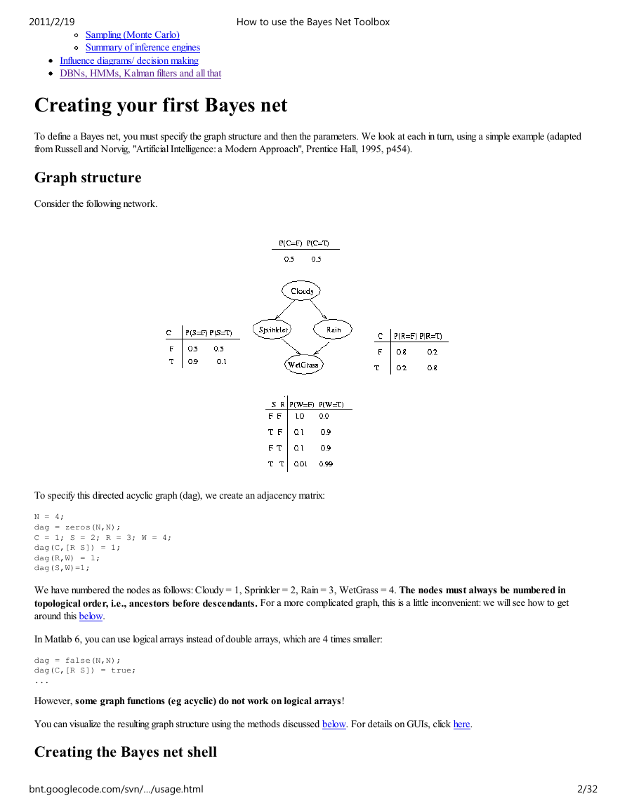
Consider the following network.
To specify this directed acyclic graph (dag), we create an adjacency matrix:
N = 4;
dag = zeros(N,N);
C = 1; S = 2; R = 3; W = 4;
dag(C,[R S]) = 1;
dag(R,W) = 1;
dag(S,W)=1;
We have numbered the nodes as follows: Cloudy = 1, Sprinkler = 2, Rain = 3, WetGrass = 4. The nodes must always be numbered in
topological order, i.e., ancestors before descendants. For a more complicated graph, this is a little inconvenient: we will see how to get
around this below.
In Matlab 6, you can use logical arrays instead of double arrays, which are 4 times smaller:
dag = false(N,N);
dag(C,[R S]) = true;
...
However, some graph functions (eg acyclic) do not work on logical arrays!
You can visualize the resulting graph structure using the methods discussed below. For details on GUIs, click here.
Creating the Bayes net shell
bnt.googlecode.com/svn/…/usage.html
2/32
�
2011/2/19
In addition to specifying the graph structure, we must specify the size and type of each node. If a node is discrete, its size is the number of
possible values each node can take on; if a node is continuous, it can be a vector, and its size is the length of this vector. In this case, we will
assume all nodes are discrete and binary.
discrete_nodes = 1:N;
node_sizes = 2*ones(1,N);
How to use the Bayes Net Toolbox
If the nodes were not binary, you could type e.g.,
node_sizes = [4 2 3 5];
meaning that Cloudy has 4 possible values, Sprinkler has 2 possible values, etc. Note that these are cardinal values, not ordinal, i.e., they are not
ordered in any way, like 'low', 'medium', 'high'.
We are now ready to make the Bayes net:
bnet = mk_bnet(dag, node_sizes, 'discrete', discrete_nodes);
By default, all nodes are assumed to be discrete, so we can also just write
bnet = mk_bnet(dag, node_sizes);
You may also specify which nodes will be observed. If you don't know, or if this not fixed in advance, just use the empty list (the default).
onodes = [];
bnet = mk_bnet(dag, node_sizes, 'discrete', discrete_nodes, 'observed', onodes);
Note that optional arguments are specified using a name/value syntax. This is common for many BNT functions. In general, to find out more about
a function (e.g., which optional arguments it takes), please see its documentation string by typing
help mk_bnet
See also other useful Matlab tips.
It is possible to associate names with nodes, as follows:
bnet = mk_bnet(dag, node_sizes, 'names', {'cloudy','S','R','W'}, 'discrete', 1:4);
You can then refer to a node by its name:
C = bnet.names('cloudy'); % bnet.names is an associative array
bnet.CPD{C} = tabular_CPD(bnet, C, [0.5 0.5]);
This feature uses my own associative array class.
Parameters
A model consists of the graph structure and the parameters. The parameters are represented by CPD objects (CPD = Conditional Probability
Distribution), which define the probability distribution of a node given its parents. (We will use the terms "node" and "random variable"
interchangeably.) The simplest kind of CPD is a table (multi-dimensional array), which is suitable when all the nodes are discrete-valued. Note
that the discrete values are not assumed to be ordered in any way; that is, they represent categorical quantities, like male and female, rather than
ordinal quantities, like low, medium and high. (We will discuss CPDs in more detail below.)
Tabular CPDs, also called CPTs (conditional probability tables), are stored as multidimensional arrays, where the dimensions are arranged in the
same order as the nodes, e.g., the CPT for node 4 (WetGrass) is indexed by Sprinkler (2), Rain (3) and then WetGrass (4) itself. Hence the
child is always the last dimension. If a node has no parents, its CPT is a column vector representing its prior. Note that in Matlab (unlike C),
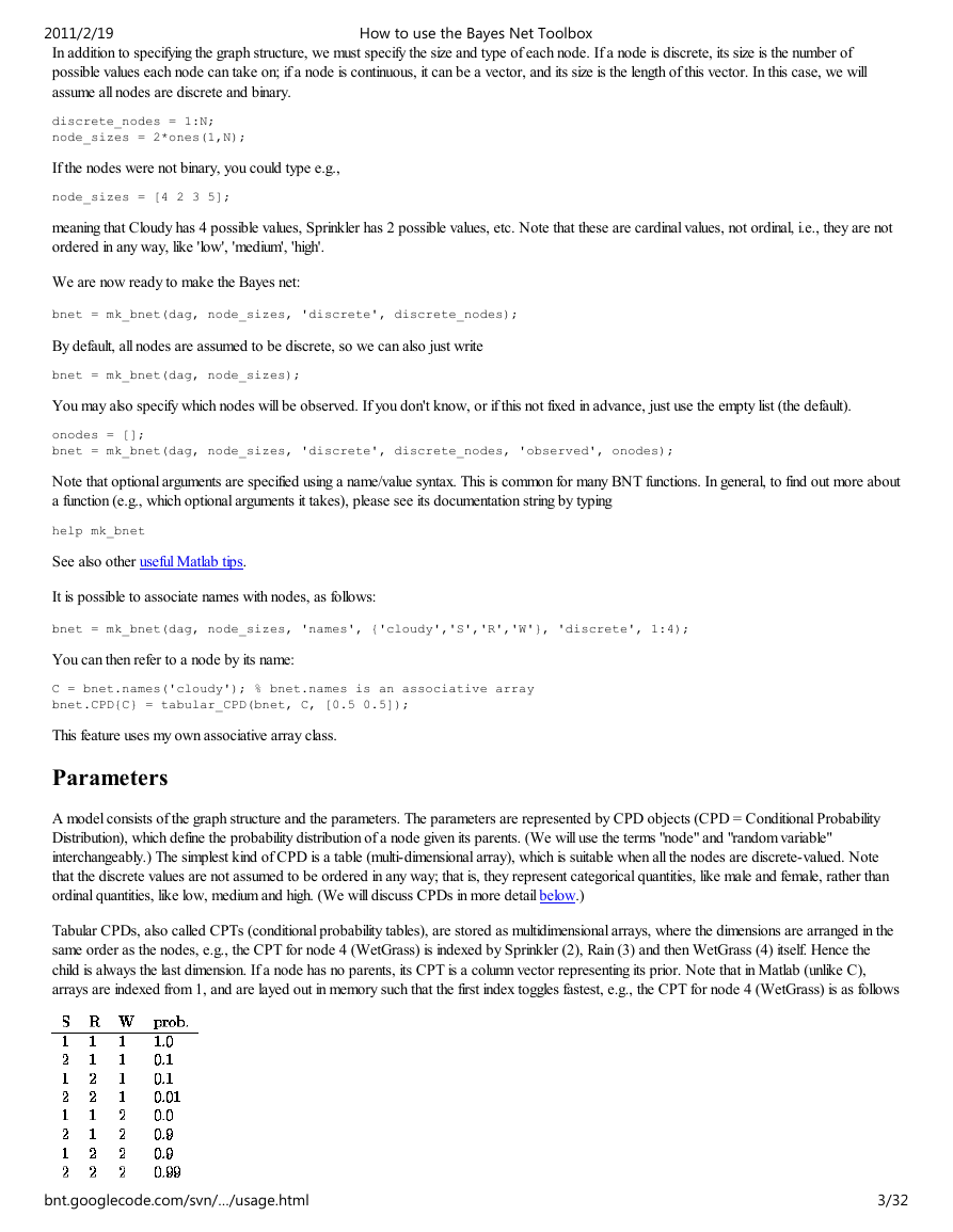
arrays are indexed from 1, and are layed out in memory such that the first index toggles fastest, e.g., the CPT for node 4 (WetGrass) is as follows
bnt.googlecode.com/svn/…/usage.html
3/32
�
2011/2/19
where we have used the convention that false==1, true==2. We can create this CPT in Matlab as follows
CPT = zeros(2,2,2);
CPT(1,1,1) = 1.0;
CPT(2,1,1) = 0.1;
...
How to use the Bayes Net Toolbox
Here is an easier way:
CPT = reshape([1 0.1 0.1 0.01 0 0.9 0.9 0.99], [2 2 2]);
In fact, we don't need to reshape the array, since the CPD constructor will do that for us. So we can just write
bnet.CPD{W} = tabular_CPD(bnet, W, 'CPT', [1 0.1 0.1 0.01 0 0.9 0.9 0.99]);
The other nodes are created similarly (using the old syntax for optional parameters)
bnet.CPD{C} = tabular_CPD(bnet, C, [0.5 0.5]);
bnet.CPD{R} = tabular_CPD(bnet, R, [0.8 0.2 0.2 0.8]);
bnet.CPD{S} = tabular_CPD(bnet, S, [0.5 0.9 0.5 0.1]);
bnet.CPD{W} = tabular_CPD(bnet, W, [1 0.1 0.1 0.01 0 0.9 0.9 0.99]);
Random Parameters
If we do not specify the CPT, random parameters will be created, i.e., each "row" of the CPT will be drawn from the uniform distribution. To
ensure repeatable results, use
rand('state', seed);
randn('state', seed);
To control the degree of randomness (entropy), you can sample each row of the CPT from a Dirichlet(p,p,...) distribution. If p << 1, this
encourages "deterministic" CPTs (one entry near 1, the rest near 0). If p = 1, each entry is drawn from U[0,1]. If p >> 1, the entries will all be
near 1/k, where k is the arity of this node, i.e., each row will be nearly uniform. You can do this as follows, assuming this node is number i, and ns
is the node_sizes.
k = ns(i);
ps = parents(dag, i);
psz = prod(ns(ps));
CPT = sample_dirichlet(p*ones(1,k), psz);
bnet.CPD{i} = tabular_CPD(bnet, i, 'CPT', CPT);
Loading a network from a file
If you already have a Bayes net represented in the XML-based Bayes Net Interchange Format (BNIF) (e.g., downloaded from the Bayes Net
repository), you can convert it to BNT format using the BIF-BNT Java program written by Ken Shan. (This is not necessarily up-to-date.)
It is currently not possible to save/load a BNT matlab object to file, but this is easily fixed if you modify all the constructors for all the
classes (see matlab documentation).
Creating a model using a GUI
Senthil Nachimuthu has started (Oct 07) an open source GUI for BNT called projeny using Java. This is a successor to BNJ.
Philippe LeRay has written (Sep 05) a BNT GUI in matlab.
LinkStrength, a package by Imme Ebert-Uphoff for visualizing the strength of dependencies between nodes.
Graph visualization
Click here for more information on graph visualization.
Inference
Having created the BN, we can now use it for inference. There are many different algorithms for doing inference in Bayes nets, that make
different tradeoffs between speed, complexity, generality, and accuracy. BNT therefore offers a variety of different inference "engines". We will
bnt.googlecode.com/svn/…/usage.html
4/32
�
2011/2/19
discuss these in more detail below. For now, we will use the junction tree engine, which is the mother of all exact inference algorithms. This can
be created as follows.
engine = jtree_inf_engine(bnet);
How to use the Bayes Net Toolbox
The other engines have similar constructors, but might take additional, algorithm-specific parameters. All engines are used in the same way, once
they have been created. We illustrate this in the following sections.
Computing marginal distributions
Suppose we want to compute the probability that the sprinker was on given that the grass is wet. The evidence consists of the fact that W=2. All
the other nodes are hidden (unobserved). We can specify this as follows.
evidence = cell(1,N);
evidence{W} = 2;
We use a 1D cell array instead of a vector to cope with the fact that nodes can be vectors of different lengths. In addition, the value [] can be
used to denote 'no evidence', instead of having to specify the observation pattern as a separate argument. (Click here for a quick tutorial on cell
arrays in matlab.)
We are now ready to add the evidence to the engine.
[engine, loglik] = enter_evidence(engine, evidence);
The behavior of this function is algorithm-specific, and is discussed in more detail below. In the case of the jtree engine, enter_evidence
implements a two-pass message-passing scheme. The first return argument contains the modified engine, which incorporates the evidence. The
second return argument contains the log-likelihood of the evidence. (Not all engines are capable of computing the log-likelihood.)
Finally, we can compute p=P(S=2|W=2) as follows.
marg = marginal_nodes(engine, S);
marg.T
ans =
0.57024
0.42976
p = marg.T(2);
We see that p = 0.4298.
Now let us add the evidence that it was raining, and see what difference it makes.
evidence{R} = 2;
[engine, loglik] = enter_evidence(engine, evidence);
marg = marginal_nodes(engine, S);
p = marg.T(2);
We find that p = P(S=2|W=2,R=2) = 0.1945, which is lower than before, because the rain can ``explain away'' the fact that the grass is wet.
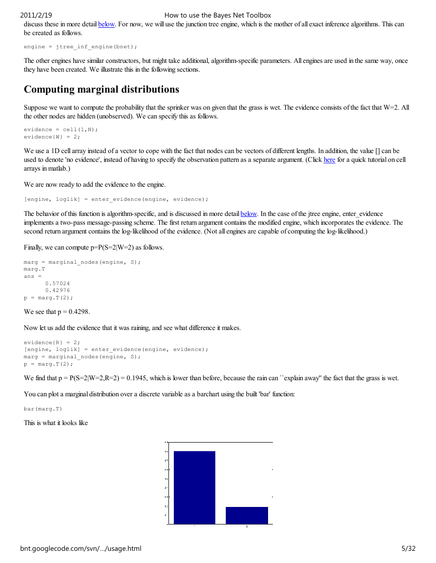
You can plot a marginal distribution over a discrete variable as a barchart using the built 'bar' function:
bar(marg.T)
This is what it looks like
bnt.googlecode.com/svn/…/usage.html
5/32
�
How to use the Bayes Net Toolbox
2011/2/19
Observed nodes
What happens if we ask for the marginal on an observed node, e.g. P(W|W=2)? An observed discrete node effectively only has 1 value (the
observed one) --- all other values would result in 0 probability. For efficiency, BNT treats observed (discrete) nodes as if they were set to 1, as
we see below:
evidence = cell(1,N);
evidence{W} = 2;
engine = enter_evidence(engine, evidence);
m = marginal_nodes(engine, W);
m.T
ans =
1
This can get a little confusing, since we assigned W=2. So we can ask BNT to add the evidence back in by passing in an optional argument:
m = marginal_nodes(engine, W, 1);
m.T
ans =
0
1
This shows that P(W=1|W=2) = 0 and P(W=2|W=2) = 1.
Computing joint distributions
We can compute the joint probability on a set of nodes as in the following example.
evidence = cell(1,N);
[engine, ll] = enter_evidence(engine, evidence);
m = marginal_nodes(engine, [S R W]);
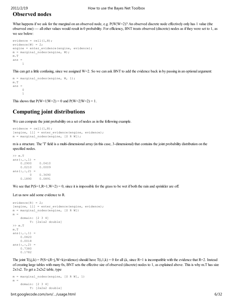
m is a structure. The 'T' field is a multi-dimensional array (in this case, 3-dimensional) that contains the joint probability distribution on the
specified nodes.
>> m.T
ans(:,:,1) =
0.2900 0.0410
0.0210 0.0009
ans(:,:,2) =
0 0.3690
0.1890 0.0891
We see that P(S=1,R=1,W=2) = 0, since it is impossible for the grass to be wet if both the rain and sprinkler are off.
Let us now add some evidence to R.
evidence{R} = 2;
[engine, ll] = enter_evidence(engine, evidence);
m = marginal_nodes(engine, [S R W])
m =
domain: [2 3 4]
T: [2x1x2 double]
>> m.T
m.T
ans(:,:,1) =
0.0820
0.0018
ans(:,:,2) =
0.7380
0.1782
The joint T(i,j,k) = P(S=i,R=j,W=k|evidence) should have T(i,1,k) = 0 for all i,k, since R=1 is incompatible with the evidence that R=2. Instead
of creating large tables with many 0s, BNT sets the effective size of observed (discrete) nodes to 1, as explained above. This is why m.T has size
2x1x2. To get a 2x2x2 table, type
m = marginal_nodes(engine, [S R W], 1)
m =
domain: [2 3 4]
T: [2x2x2 double]
bnt.googlecode.com/svn/…/usage.html
6/32
�
How to use the Bayes Net Toolbox
2011/2/19
>> m.T
m.T
ans(:,:,1) =
0 0.082
0 0.0018
ans(:,:,2) =
0 0.738
0 0.1782
Note: It is not always possible to compute the joint on arbitrary sets of nodes: it depends on which inference engine you use, as discussed in more
detail below.
Soft/virtual evidence
Sometimes a node is not observed, but we have some distribution over its possible values; this is often called "soft" or "virtual" evidence. One can
use this as follows
[engine, loglik] = enter_evidence(engine, evidence, 'soft', soft_evidence);
where soft_evidence{i} is either [] (if node i has no soft evidence) or is a vector representing the probability distribution over i's possible values.
For example, if we don't know i's exact value, but we know its likelihood ratio is 60/40, we can write evidence{i} = [] and soft_evidence{i} =
[0.6 0.4].
Currently only jtree_inf_engine supports this option. It assumes that all hidden nodes, and all nodes for which we have soft evidence, are discrete.
For a longer example, see BNT/examples/static/softev1.m.
Most probable explanation
To compute the most probable explanation (MPE) of the evidence (i.e., the most probable assignment, or a mode of the joint), use
[mpe, ll] = calc_mpe(engine, evidence);
mpe{i} is the most likely value of node i. This calls enter_evidence with the 'maximize' flag set to 1, which causes the engine to do max-product
instead of sum-product. The resulting max-marginals are then thresholded. If there is more than one maximum probability assignment, we must
take care to break ties in a consistent manner (thresholding the max-marginals may give the wrong result). To force this behavior, type
[mpe, ll] = calc_mpe(engine, evidence, 1);
Note that computing the MPE is someties called abductive reasoning.
You can also use calc_mpe_bucket written by Ron Zohar, that does a forwards max-product pass, and then a backwards traceback pass,
which is how Viterbi is traditionally implemented.
Conditional Probability Distributions
A Conditional Probability Distributions (CPD) defines P(X(i) | X(Pa(i))), where X(i) is the i'th node, and X(Pa(i)) are the parents of node i. There
are many ways to represent this distribution, which depend in part on whether X(i) and X(Pa(i)) are discrete, continuous, or a combination. We
will discuss various representations below.
Tabular nodes
If the CPD is represented as a table (i.e., if it is a multinomial distribution), it has a number of parameters that is exponential in the number of
parents. See the example above.
Noisy-or nodes
A noisy-OR node is like a regular logical OR gate except that sometimes the effects of parents that are on get inhibited. Let the prob. that parent i
gets inhibited be q(i). Then a node, C, with 2 parents, A and B, has the following CPD, where we use F and T to represent off and on (1 and 2 in
BNT).
A B P(C=off) P(C=on)
---------------------------
bnt.googlecode.com/svn/…/usage.html
7/32
�
2011/2/19
F F 1.0 0.0
T F q(A) 1-q(A)
F T q(B) 1-q(B)
T T q(A)q(B) 1-q(A)q(B)
How to use the Bayes Net Toolbox
Thus we see that the causes get inhibited independently. It is common to associate a "leak" node with a noisy-or CPD, which is like a parent that
is always on. This can account for all other unmodelled causes which might turn the node on.
The noisy-or distribution is similar to the logistic distribution. To see this, let the nodes, S(i), have values in {0,1}, and let q(i,j) be the prob. that j
inhibits i. Then
Pr(S(i)=1 | parents(S(i))) = 1 - prod_{j} q(i,j)^S(j)
Now define w(i,j) = -ln q(i,j) and rho(x) = 1-exp(-x). Then
Pr(S(i)=1 | parents(S(i))) = rho(sum_j w(i,j) S(j))
For a sigmoid node, we have
Pr(S(i)=1 | parents(S(i))) = sigma(-sum_j w(i,j) S(j))
where sigma(x) = 1/(1+exp(-x)). Hence they differ in the choice of the activation function (although both are monotonically increasing). In
addition, in the case of a noisy-or, the weights are constrained to be positive, since they derive from probabilities q(i,j). In both cases, the number
of parameters is linear in the number of parents, unlike the case of a multinomial distribution, where the number of parameters is exponential in
the number of parents. We will see an example of noisy-OR nodes below.
Other (noisy) deterministic nodes
Deterministic CPDs for discrete random variables can be created using the deterministic_CPD class. It is also possible to 'flip' the output of the
function with some probability, to simulate noise. The boolean_CPD class is just a special case of a deterministic CPD, where the parents and
child are all binary.
Both of these classes are just "syntactic sugar" for the tabular_CPD class.
Softmax nodes
If we have a discrete node with a continuous parent, we can define its CPD using a softmax function (also known as the multinomial logit
function). This acts like a soft thresholding operator, and is defined as follows:
exp(w(:,i)'*x + b(i))
Pr(Q=i | X=x) = -----------------------------
sum_j exp(w(:,j)'*x + b(j))
The parameters of a softmax node, w(:,i) and b(i), i=1..|Q|, have the following interpretation: w(:,i)-w(:,j) is the normal vector to the decision
boundary between classes i and j, and b(i)-b(j) is its offset (bias). For example, suppose X is a 2-vector, and Q is binary. Then
w = [1 -1;
0 0];
b = [0 0];
means class 1 are points in the 2D plane with positive x coordinate, and class 2 are points in the 2D plane with negative x coordinate. If w has
large magnitude, the decision boundary is sharp, otherwise it is soft. In the special case that Q is binary (0/1), the softmax function reduces to the
logistic (sigmoid) function.
Fitting a softmax function can be done using the iteratively reweighted least squares (IRLS) algorithm. We use the implementation from Netlab.
Note that since the softmax distribution is not in the exponential family, it does not have finite sufficient statistics, and hence we must store all the
training data in uncompressed form. If this takes too much space, one should use online (stochastic) gradient descent (not implemented in BNT).
If a softmax node also has discrete parents, we use a different set of w/b parameters for each combination of parent values, as in the conditional
linear Gaussian CPD. This feature was implemented by Pierpaolo Brutti. He is currently extending it so that discrete parents can be treated as if
they were continuous, by adding indicator variables to the X vector.
We will see an example of softmax nodes below.
bnt.googlecode.com/svn/…/usage.html
8/32
�





 2023年江西萍乡中考道德与法治真题及答案.doc
 2012年重庆南川中考生物真题及答案.doc
 2013年江西师范大学地理学综合及文艺理论基础考研真题.doc
 2020年四川甘孜小升初语文真题及答案I卷.doc
 2020年注册岩土工程师专业基础考试真题及答案.doc
 2023-2024学年福建省厦门市九年级上学期数学月考试题及答案.doc
 2021-2022学年辽宁省沈阳市大东区九年级上学期语文期末试题及答案.doc
 2022-2023学年北京东城区初三第一学期物理期末试卷及答案.doc
 2018上半年江西教师资格初中地理学科知识与教学能力真题及答案.doc
 2012年河北国家公务员申论考试真题及答案-省级.doc
 2020-2021学年江苏省扬州市江都区邵樊片九年级上学期数学第一次质量检测试题及答案.doc
 2022下半年黑龙江教师资格证中学综合素质真题及答案.doc