An Introduction to Physically Based Modeling:
Rigid Body Simulation I—Unconstrained Rigid Body
Dynamics
David Baraff
Robotics Institute
Carnegie Mellon University
Please note: This document is ª 1997 by David Baraff. This chapter may be freely
duplicated and distributed so long as no consideration is received in return, and this
copyright notice remains intact.
�
Rigid Body Simulation
David Baraff
Robotics Institute
Carnegie Mellon University
Introduction
This portion of the course notes deals with the problem of rigid body dynamics. To help get you
started simulating rigid body motion, we’ve provided code fragments that implement most of the
concepts discussed in these notes. This segment of the course notes is divided into two parts. The first
part covers the motion of rigid bodies that are completely unconstrained in their allowable motion;
that is, simulations that aren’t concerned about collisions between rigid bodies. Given any external
forces acting on a rigid body, we’ll show how to simulate the motion of the body in response to these
forces. The mathematical derivations in these notes are meant to be fairly informal and intuitive.
The second part of the notes tackles the problem of constrained motion that arises when we
regard bodies as solid, and need to disallow inter-penetration. We enforce these non-penetration
constraints by computing appropriate contact forces between contacting bodies. Given values for
these contact forces, simulation proceeds exactly as in the unconstrained case: we simply apply all
the forces to the bodies and let the simulation unfold as though the motions of bodies are completely
unconstrained. If we have computed the contact forces correctly, the resulting motion of the bodies
will be free from inter-penetration. The computation of these contact forces is the most demanding
component of the entire simulation process.1
1Collision detection (i.e. determining the points of contact between bodies) runs a close second though!
D1
�
Part I. Unconstrained Rigid Body Dynamics
1 Simulation Basics
This portion of the course notes is geared towards a full implementation of rigid body motion. In this
section, we’ll show the basic structure for simulating the motion of a rigid body. In section 2, we’ll
define the terms, concepts, and equations we need to implement a rigid body simulator. Following
this, we’ll give some code to actually implement the equations we need. Derivations for some of the
concepts and equations we will be using will be left to appendix A.
The only thing you need to be familiar with at this point are the basic concepts (but not the numer-
ical details) of solving ordinary differential equations. If you’re not familiar with this topic, you’re
in luck: just turn back to the beginning of these course notes, and read the section on “Differential
Equation Basics.” You also might want to read the next section on “Particle Dynamics” as well,
although we’re about to repeat some of that material here anyway.
Simulating the motion of a rigid body is almost the same as simulating the motion of a particle,
so let’s start with particle simulation. The way we simulate a particle is as follows. We let a function
x.t/ denote the particle’s location in world space (the space all particles or bodies occupy during
simulation) at time t. The function v.t/ D Px.t/ D d
dt x.t/ gives the velocity of the particle at time t.
The state of a particle at time t is the particle’s position and velocity. We generalize this concept by
defining a state vector Y.t/ for a system: for a single particle,
Y.t/ D
x.t/
v.t/
:
(1–1)
When we’re talking about an actual implementation, we have to “flatten” out Y.t/ into an array.
For a single particle, Y.t/ can be described as an array of six numbers: typically, we’d let the first
three elements of the array represent x.t/, and the last three elements represent v.t/. Later, when we
talk about state vectors Y.t/ that contain matrices as well as vectors, the same sort of operation is
done to flatten Y.t/ into an array. Of course, we’ll also have to reverse this process and turn an array
of numbers back into a state vector Y.t/. This all comes down to pretty simple bookkeeping though,
so henceforth, we’ll assume that we know how to convert any sort of state vector Y.t/ to an array
(of the appropriate length) and vice versa. (For a simple example involving particles, look through
the “Particle System Dynamics” section of these notes.)
For a system with n particles, we enlarge Y.t/ to be
0BBBBB@
Y.t/ D
1CCCCCA
x1.t/
v1.t/
...
xn.t/
vn.t/
(1–2)
SIGGRAPH ’97 COURSE NOTES
D2
PHYSICALLY BASED MODELING
�
where xi.t/ and vi.t/ are the position and velocity of the ith particle. Working with n particles is no
harder than working with one particle, so we’ll let Y.t/ be the state vector for a single particle for
now (and when we get to it later, a single rigid body).
To actually simulate the motion of our particle, we need to know one more thing—the force
acting on the particle at time t. We’ll define F.t/ as the force acting on our particle at time t. The
function F.t/ is the sum of all the forces acting on the particle: gravity, wind, spring forces, etc. If
the particle has mass m, then the change of Y over time is given by
d
dt
Y.t/ D d
dt
x.t/
v.t/
D
v.t/
F.t/=m
:
(1–3)
Given any value of Y.t/, equation (1–3) describes how Y.t/ is instantaneously changing at time t.
A simulation starts with some initial conditions for Y.0/, (i.e. values for x.0/ and v.0/) and then
uses a numerical equation solver to track the change or “flow” of Y over time, for as long as we’re
interested in. If all we want to know is the particle’s location one second from now, we ask the solver
to compute Y.1/, assuming that time units are in seconds. If we’re going to animate the motion of
the particle, we’d want to compute Y. 1
30
The numerical method used by the solver is relatively unimportant with respect to our actual
implementation. Let’s look at how we’d actually interact with a numerical solver, in a C++-like
language. Assume we have access to a numerical solver, which we’ll generically write as a function
named ode. Typically, ode has the following specification:
/, Y. 2
30
/ and so on.
typedef void �*dydt_func��double t, double y� �, double ydot� ��;
void
ode�double y�� �, double yend� �, int len, double t�,
double t�, dydt_func dydt�;
We pass an initial state vector to ode as an array y�. The solver ode knows nothing about the
inherent structure of y�. Since solvers can handle problems of arbitrary dimension, we also have to
pass the length len of y�. (For a system of n particles, we’d obviously have len D 6n.) We also
pass the solver the starting and ending times of the simulation, t� and t�. The solver’s goal is to
compute the state vector at time t� and return it in the array yend.
We also pass a function dydt to ode. Given an array y that encodes a state vector Y.t/ and a
time t, dydt must compute and return d
dtY.t/ in the array ydot. (The reason we must pass t to dydt
is that we may have time-varying forces acting in our system. In that case, dydt would have to know
“what time it is” to determine the value of those forces.) In tracing the flow of Y.t/ from t� to t�,
the solver ode is allowed to call dydt as often as it likes. Given that we have such a routine ode,
the only work we need to do is to code up the routine dydt which we’ll give as a parameter to ode.
Simulating rigid bodies follows exactly the same mold as simulating particles. The only differ-
ence is that the state vector Y.t/ for a rigid body holds more information, and the derivatived
dtY.t/ is
a little more complicated. However, we’ll use exactly the same paradigm of tracking the movement
of a rigid body using a solver ode, which we’ll supply with a function dydt.
2 Rigid Body Concepts
The goal of this section is to develop an analogue to equation (1–3), for rigid bodies. The final
differential equation we develop is given in section 2.11. In order to do this though, we need to define
SIGGRAPH ’97 COURSE NOTES
D3
PHYSICALLY BASED MODELING
�
a lot of concepts first and relations first. Some of the longer derivations are found in appendix A. In
the next section, we’ll show how to write the function dydt needed by the numerical solver ode to
compute the derivative d
dtY.t/ developed in this section.
2.1 Position and Orientation
The location of a particle in space at time t can be described as a vector x.t/, which describes the
translation of the particle from the origin. Rigid bodies are more complicated, in that in addition to
translating them, we can also rotate them. To locate a rigid body in world space, we’ll use a vector
x.t/, which describes the translation of the body. We must also describe the rotation of the body,
which we’ll do (for now) in terms of a 3 3 rotation matrix R.t/. We will call x.t/ and R.t/ the
spatial variables of a rigid body.
A rigid body, unlike a particle, occupies a volume of space and has a particular shape. Because a
rigid body can undergo only rotation and translation, we define the shape of a rigid body in terms of
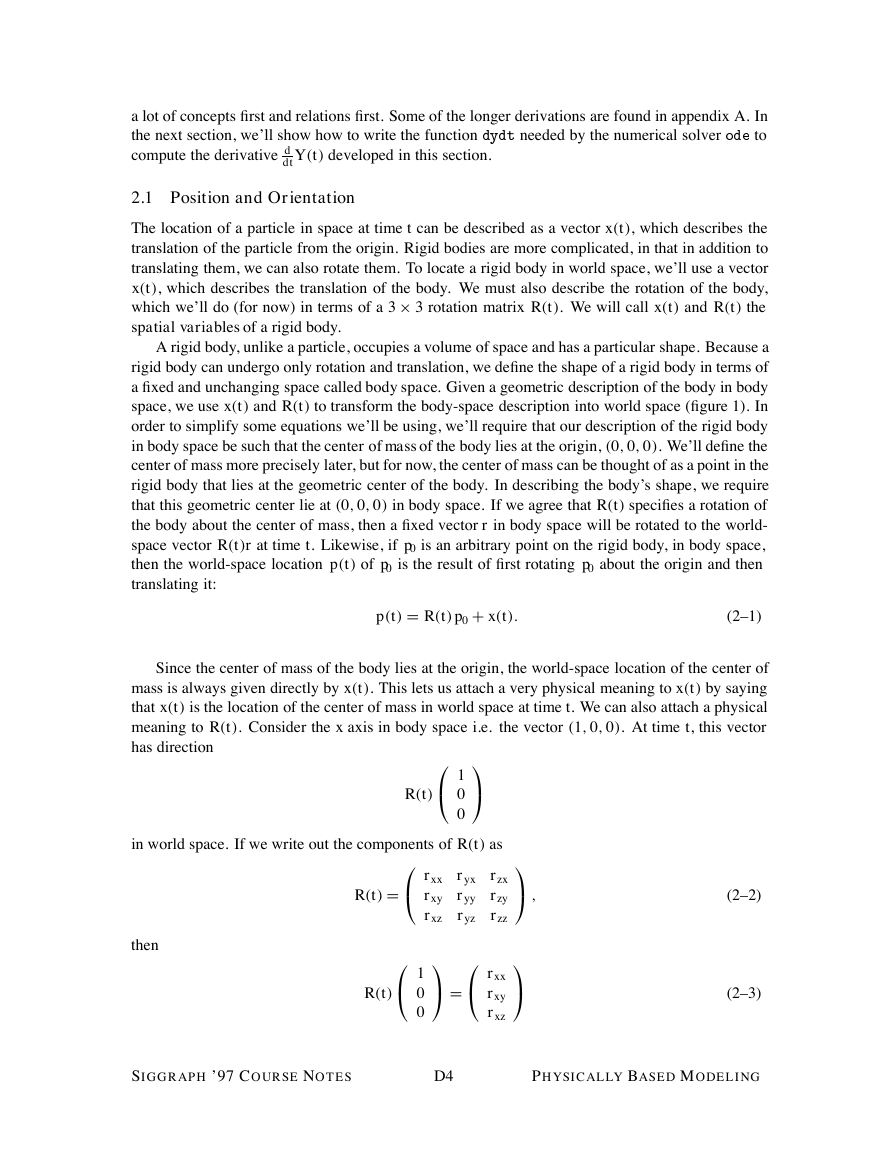
a fixed and unchanging space called body space. Given a geometric description of the body in body
space, we use x.t/ and R.t/ to transform the body-space description into world space (figure 1). In
order to simplify some equations we’ll be using, we’ll require that our description of the rigid body
in body space be such that the center of mass of the body lies at the origin, .0; 0; 0/. We’ll define the
center of mass more precisely later, but for now, the center of mass can be thought of as a point in the
rigid body that lies at the geometric center of the body. In describing the body’s shape, we require
that this geometric center lie at .0; 0; 0/ in body space. If we agree that R.t/ specifies a rotation of
the body about the center of mass, then a fixed vector r in body space will be rotated to the world-
space vector R.t/r at time t. Likewise, if p0 is an arbitrary point on the rigid body, in body space,
then the world-space location p.t/ of p0 is the result of first rotating p0 about the origin and then
translating it:
p.t/ D R.t/ p0 C x.t/:
(2–1)
Since the center of mass of the body lies at the origin, the world-space location of the center of
mass is always given directly by x.t/. This lets us attach a very physical meaning to x.t/ by saying
that x.t/ is the location of the center of mass in world space at time t. We can also attach a physical
meaning to R.t/. Consider the x axis in body space i.e. the vector .1; 0; 0/. At time t, this vector
has direction
0
0
R.t/
0@ 1
0@ rxx
1A D
0@ 1
rxy
rxz
0
0
R.t/ D
1A
ryx
ryy
ryz
rzx
rzy
rzz
0@ rxx
rxy
rxz
1A ;
1A
(2–2)
(2–3)
in world space. If we write out the components of R.t/ as
then
R.t/
SIGGRAPH ’97 COURSE NOTES
D4
PHYSICALLY BASED MODELING
�
body space
world space
y'
y
0
z
p0
x
y
x(t)
z
x
z'
p(t)
x'
Figure 1: The center of mass is transformed to the point x.t/ in world space, at time t. The fixed x, y,
0 D R.t/z.
and z axes of the body in body space transform to the vectors x
The fixed point p0 in body space is transformed to the point p.t/ D R.t/ p0 C x.t/.
0 D R.t/y and z
0 D R.t/x, y
which is the first column of R.t/. The physical meaning of R.t/ is that R.t/’s first column gives the
direction that the rigid body’s x axis points in, when transformed to world space at time t. Similarly,
the second and third columns of R.t/,0@ ryx
1A
1A
0@ rzx
rzy
rzz
ryy
ryz
and
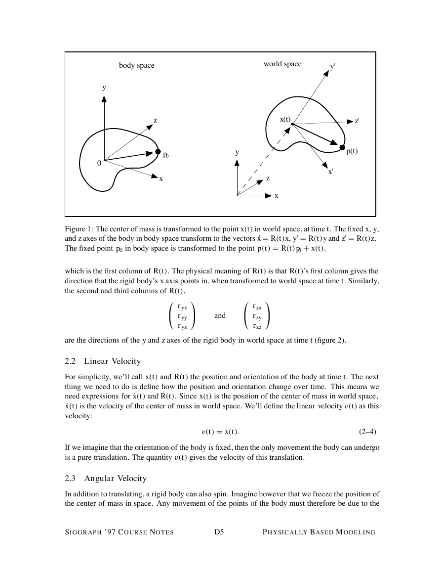
are the directions of the y and z axes of the rigid body in world space at time t (figure 2).
2.2 Linear Velocity
For simplicity, we’ll call x.t/ and R.t/ the position and orientation of the body at time t. The next
thing we need to do is define how the position and orientation change over time. This means we
need expressions for Px.t/ and PR.t/. Since x.t/ is the position of the center of mass in world space,
Px.t/ is the velocity of the center of mass in world space. We’ll define the linear velocity v.t/ as this
velocity:
v.t/ D Px.t/:
(2–4)
If we imagine that the orientation of the body is fixed, then the only movement the body can undergo
is a pure translation. The quantity v.t/ gives the velocity of this translation.
2.3 Angular Velocity
In addition to translating, a rigid body can also spin. Imagine however that we freeze the position of
the center of mass in space. Any movement of the points of the body must therefore be due to the
SIGGRAPH ’97 COURSE NOTES
D5
PHYSICALLY BASED MODELING
�
R(t) = [ x' y' z' ]
world space
y'
z'
x'
y
z
x
Figure 2: Physical interpretation of the orientation matrix R.t/. At time t, the columns of R.t/ are
the world-space directions that the body-space x, y, and z axes transform to.
body spinning about some axis that passes through the center of mass. (Otherwise the center of mass
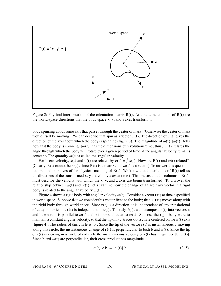
would itself be moving). We can describe that spin as a vector !.t/. The direction of !.t/ gives the
direction of the axis about which the body is spinning (figure 3). The magnitude of !.t/, j!.t/j, tells
how fast the body is spinning. j!.t/j has the dimensions of revolutions/time; thus, j!.t/j relates the
angle through which the body will rotate over a given period of time, if the angular velocity remains
constant. The quantity !.t/ is called the angular velocity.
For linear velocity, x.t/ and v.t/ are related by v.t/ D d
dt x.t/. How are R.t/ and !.t/ related?
(Clearly, PR.t/ cannot be !.t/, since R.t/ is a matrix, and !.t/ is a vector.) To answer this question,
let’s remind ourselves of the physical meaning of R.t/. We know that the columns of R.t/ tell us
the directions of the transformed x, y and z body axes at time t. That means that the columns ofPR.t/
must describe the velocity with which the x, y, and z axes are being transformed. To discover the
relationship between !.t/ and R.t/, let’s examine how the change of an arbitrary vector in a rigid
body is related to the angular velocity !.t/.
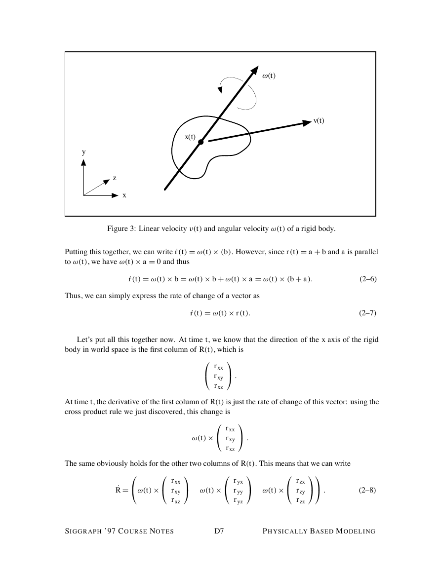
Figure 4 shows a rigid body with angular velocity !.t/. Consider a vector r.t/ at time t specified
in world space. Suppose that we consider this vector fixed to the body; that is, r.t/ moves along with
the rigid body through world space. Since r.t/ is a direction, it is independent of any translational
effects; in particular, Pr.t/ is independent of v.t/. To study Pr.t/, we decompose r.t/ into vectors a
and b, where a is parallel to !.t/ and b is perpendicular to !.t/. Suppose the rigid body were to
maintain a constant angular velocity, so that the tip of r.t/ traces out a circle centered on the !.t/ axis
(figure 4). The radius of this circle is jbj. Since the tip of the vector r.t/ is instantaneously moving
along this circle, the instantaneous change of r.t/ is perpendicular to both b and !.t/. Since the tip
of r.t/ is moving in a circle of radius b, the instantaneous velocity of r.t/ has magnitude jbjj!.t/j.
Since b and !.t/ are perpendicular, their cross product has magnitude
j!.t/ bj D j!.t/jjbj:
(2–5)
SIGGRAPH ’97 COURSE NOTES
D6
PHYSICALLY BASED MODELING
�
w (t)
v(t)
x(t)
y
z
x
Figure 3: Linear velocity v.t/ and angular velocity !.t/ of a rigid body.
Putting this together, we can write Pr.t/ D !.t/ .b/. However, since r.t/ D a C b and a is parallel
to !.t/, we have !.t/ a D 0 and thus
Pr.t/ D !.t/ b D !.t/ b C !.t/ a D !.t/ .b C a/:
Thus, we can simply express the rate of change of a vector as
Pr.t/ D !.t/ r.t/:
(2–6)
(2–7)
Let’s put all this together now. At time t, we know that the direction of the x axis of the rigid
body in world space is the first column of R.t/, which is
At time t, the derivative of the first column of R.t/ is just the rate of change of this vector: using the
cross product rule we just discovered, this change is
rxy
rxz
0@ rxx
1A :
1A :
0@ rxx
0@ ryx
1A !.t/
1A !.t/
!.t/
rxy
rxz
ryy
ryz
The same obviously holds for the other two columns of R.t/. This means that we can write
0@!.t/
0@ rxx
rxy
rxz
PR D
1A1A :
0@ rzx
rzy
rzz
(2–8)
SIGGRAPH ’97 COURSE NOTES
D7
PHYSICALLY BASED MODELING
�


 2023年江西萍乡中考道德与法治真题及答案.doc
 2012年重庆南川中考生物真题及答案.doc
 2013年江西师范大学地理学综合及文艺理论基础考研真题.doc
 2020年四川甘孜小升初语文真题及答案I卷.doc
 2020年注册岩土工程师专业基础考试真题及答案.doc
 2023-2024学年福建省厦门市九年级上学期数学月考试题及答案.doc
 2021-2022学年辽宁省沈阳市大东区九年级上学期语文期末试题及答案.doc
 2022-2023学年北京东城区初三第一学期物理期末试卷及答案.doc
 2018上半年江西教师资格初中地理学科知识与教学能力真题及答案.doc
 2012年河北国家公务员申论考试真题及答案-省级.doc
 2020-2021学年江苏省扬州市江都区邵樊片九年级上学期数学第一次质量检测试题及答案.doc
 2022下半年黑龙江教师资格证中学综合素质真题及答案.doc