EUROGRAPHICS 2003 / P.Brunet and D. Fellner Volume 22 (2003), Number 3
(Guest Editors)
Multi-scale Feature Extraction on Point-sampled Surfaces
Mark Pauly Richard Keiser Markus Gross
ETH Zürich
Abstract
We present a new technique for extracting line-type features on point-sampled geometry. Given an unstruc-
tured point cloud as input, our method first applies principal component analysis on local neighborhoods to
classify points according to the likelihood that they belong to a feature. Using hysteresis thresholding, we then
compute a minimum spanning graph as an initial approximation of the feature lines. To smooth out the features
while maintaining a close connection to the underlying surface, we use an adaptation of active contour mod-
els. Central to our method is a multi-scale classification operator that allows feature analysis at multiple
scales, using the size of the local neighborhoods as a discrete scale parameter. This significantly improves the
reliability of the detection phase and makes our method more robust in the presence of noise. To illustrate the
usefulness of our method, we have implemented a non-photorealistic point renderer to visualize point-sampled
surfaces as line drawings of their extracted feature curves.
1. Introduction
Point-sampled surfaces have emerged in recent years as a
versatile representation for geometric models in computer
graphics. The surface of a 3D object is described by a set of
sample points without further topological information such
as triangle mesh connectivity or a parameterization. Reduc-
ing the representation to the essentials, i.e. the geometric
position of the sample points, is particularly useful when
dealing with large data sets generated by modern acquisi-
tion devices [15]. To display such models, numerous point-
based rendering systems have been developed, e.g. [20, 21,
25, 1]. Apart from acquisition and rendering, a variety of
geometry processing applications have been introduced
recently [18, 19, 26] that demonstrate the versatility of
points as a geometric modeling primitive.
In this paper, we present a new method for detecting and
extracting line-type features on point-sampled surfaces.
This type of information can serve as input for many pro-
cessing applications such as meshing, model segmentation,
or anisotropic fairing. Feature lines can also be used for
visualization to enhance the semantics of renditions of 3D
objects. In Section 4 we will show how artistic line draw-
ings of point-sampled surfaces can be created using the
extracted feature curves.
Features are usually defined as entities of an object that
are considered important by a human for an accurate
description of the object. This definition is highly subjec-
tive, however, and very difficult to express in algorithmic
form. Our goal was to design a feature extraction algorithm
that requires no additional semantic information about the
object. Also, our method should be semi-automatic, i.e.
only require the user to specify a few thresholding parame-
ters. Additional interaction with the object, such as setting
seed points or guiding feature movement, is not necessary.
We therefore base our feature definition on low-level infor-
mation using a statistical operator that measures local sur-
face variation. This operator classifies points according to
the likelihood that they belong to a feature. To improve the
robustness and reliability of the classification stage, we
apply this operator at multiple scales, which allows us to
measure the persistence of a feature [4]. Additionally,
multi-scale classification provides further structural infor-
mation per classified point, e.g. the characteristic scale at
which a feature is most prominent.
We concentrate on line-type features. These are probably
the most important features for surfaces, which are often
composed of patches that are framed by feature lines. A fea-
ture line approximately passes along a ridge of maximum
inflection, which is adequately captured in our surface vari-
ation estimate.
We believe that low-level feature extraction methods
such as ours always require some user feedback, in particu-
lar for our example application of an artistic line-drawing
renderer. To obtain visually pleasing renditions, the user has
to adjust the various parameters of our feature extraction
method until she is satisfied with the result. We therefore
�
Pauly, Keiser, Gross / Multi-scale Feature Extraction on Point-sampled Surfaces
input
point cloud
multi-scale
classification
hysteresis
thresholding
MSG
construction
feature
smoothing
line art
rendering
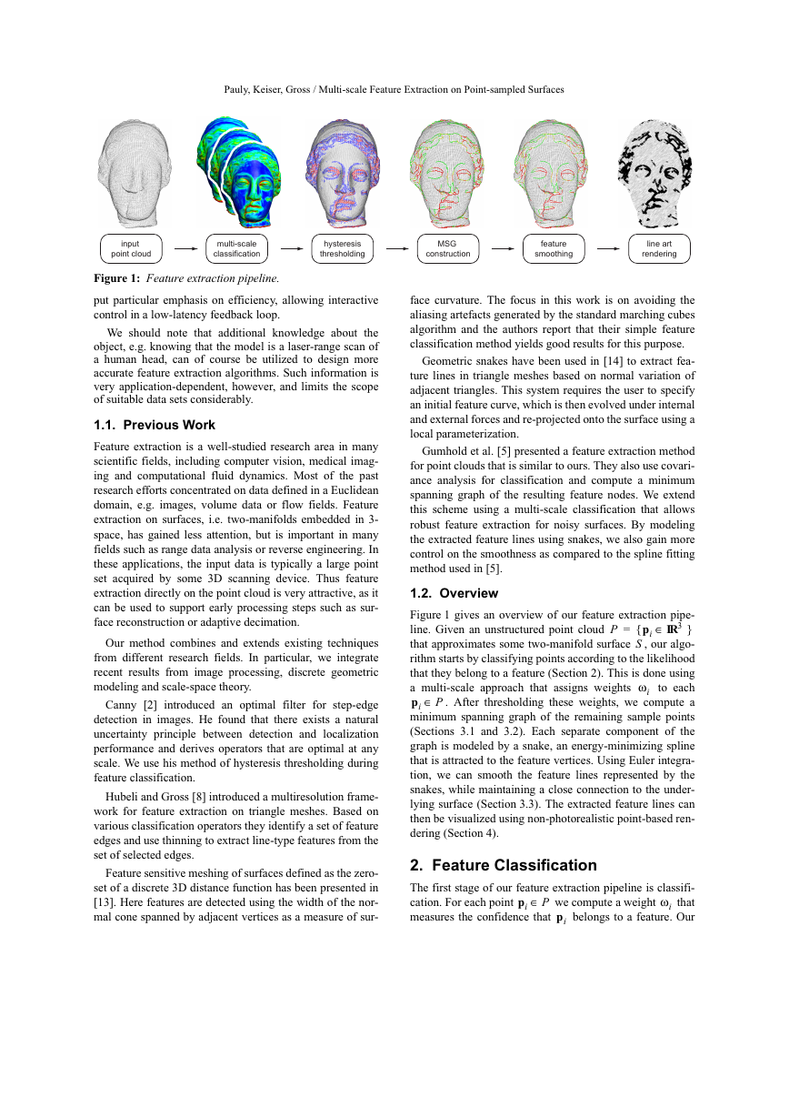
Figure 1: Feature extraction pipeline.
put particular emphasis on efficiency, allowing interactive
control in a low-latency feedback loop.
We should note that additional knowledge about the
object, e.g. knowing that the model is a laser-range scan of
a human head, can of course be utilized to design more
accurate feature extraction algorithms. Such information is
very application-dependent, however, and limits the scope
of suitable data sets considerably.
1.1. Previous Work
Feature extraction is a well-studied research area in many
scientific fields, including computer vision, medical imag-
ing and computational fluid dynamics. Most of the past
research efforts concentrated on data defined in a Euclidean
domain, e.g. images, volume data or flow fields. Feature
extraction on surfaces, i.e. two-manifolds embedded in 3-
space, has gained less attention, but is important in many
fields such as range data analysis or reverse engineering. In
these applications, the input data is typically a large point
set acquired by some 3D scanning device. Thus feature
extraction directly on the point cloud is very attractive, as it
can be used to support early processing steps such as sur-
face reconstruction or adaptive decimation.
Our method combines and extends existing techniques
from different research fields. In particular, we integrate
recent results from image processing, discrete geometric
modeling and scale-space theory.
Canny [2] introduced an optimal filter for step-edge
detection in images. He found that there exists a natural
uncertainty principle between detection and localization
performance and derives operators that are optimal at any
scale. We use his method of hysteresis thresholding during
feature classification.
Hubeli and Gross [8] introduced a multiresolution frame-
work for feature extraction on triangle meshes. Based on
various classification operators they identify a set of feature
edges and use thinning to extract line-type features from the
set of selected edges.
Feature sensitive meshing of surfaces defined as the zero-
set of a discrete 3D distance function has been presented in
[13]. Here features are detected using the width of the nor-
mal cone spanned by adjacent vertices as a measure of sur-
face curvature. The focus in this work is on avoiding the
aliasing artefacts generated by the standard marching cubes
algorithm and the authors report that their simple feature
classification method yields good results for this purpose.
Geometric snakes have been used in [14] to extract fea-
ture lines in triangle meshes based on normal variation of
adjacent triangles. This system requires the user to specify
an initial feature curve, which is then evolved under internal
and external forces and re-projected onto the surface using a
local parameterization.
Gumhold et al. [5] presented a feature extraction method
for point clouds that is similar to ours. They also use covari-
ance analysis for classification and compute a minimum
spanning graph of the resulting feature nodes. We extend
this scheme using a multi-scale classification that allows
robust feature extraction for noisy surfaces. By modeling
the extracted feature lines using snakes, we also gain more
control on the smoothness as compared to the spline fitting
method used in [5].
P
1.2. Overview
Figure 1 gives an overview of our feature extraction pipe-
IR3∈{
}
pi
line. Given an unstructured point cloud
=
that approximates some two-manifold surface
, our algo-
S
rithm starts by classifying points according to the likelihood
that they belong to a feature (Section 2). This is done using
a multi-scale approach that assigns weights
to each
pi P∈
. After thresholding these weights, we compute a
minimum spanning graph of the remaining sample points
(Sections 3.1 and 3.2). Each separate component of the
graph is modeled by a snake, an energy-minimizing spline
that is attracted to the feature vertices. Using Euler integra-
tion, we can smooth the feature lines represented by the
snakes, while maintaining a close connection to the under-
lying surface (Section 3.3). The extracted feature lines can
then be visualized using non-photorealistic point-based ren-
dering (Section 4).
ω
i
2. Feature Classification
The first stage of our feature extraction pipeline is classifi-
pi P∈
cation. For each point
that
measures the confidence that
belongs to a feature. Our
we compute a weight
pi
ω
i
�
Pauly, Keiser, Gross / Multi-scale Feature Extraction on Point-sampled Surfaces
feature classification is based on surface variation estima-
tion using covariance analysis of local neighborhoods. We
will show how this statistical approach can be incorporated
into a scale-space framework that allows feature classifica-
tion at multiple scales.
2.1. Scale Space
Since their introduction in 1983 [24], scale-space represen-
tations have been studied extensively in the context of fea-
ture detection for images. The fundamental idea is to model
at
a
as
L : IR d
is defined as a convolution
L
of varying width
of
IR→
, where
G
with Gaussian kernels
f : IRd
IR→
signal
×
different
scales
IR +
:
t
f
L x t,(
)
=
G x t,(
)
⊗
f x( )
IR d∈
x
with
(see Figure 2). Equivalently,
defined as the solution of the diffusion equation
L∂
t∂------
=
1
---∇2L
2
.
(1)
L
can be
(2)
Given a scale-space representation
, we can then
apply a classification operator to measure the desired func-
tion properties, e.g. curvature, at different scales.
L x t,(
)
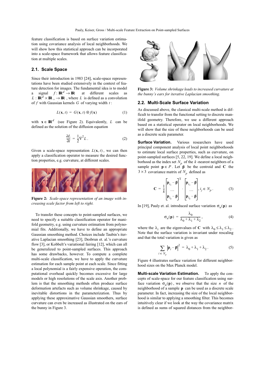
Figure 2: Scale-space representation of an image with in-
creasing scale factor from left to right.
To transfer these concepts to point-sampled surfaces, we
need to specify a suitable classification operator for mani-
fold geometry, e.g. using curvature estimation from polyno-
mial fits. Additionally, we have to define an appropriate
Gaussian smoothing method. Choices include Taubin’s iter-
ative Laplacian smoothing [23], Desbrun et. al.’s curvature
flow [3], or Kobbelt’s variational fairing [12], which can all
be generalized to point-sampled surfaces. This approach
has some drawbacks, however. To compute a complete
multi-scale classification, we have to apply the curvature
estimation for each sample point at each scale. Since fitting
a local polynomial is a fairly expensive operation, the com-
putational overhead quickly becomes excessive for large
models or high resolutions of the scale axis. Another prob-
lem is that the smoothing methods often produce surface
deformation artefacts such as volume shrinkage, caused by
inevitable distortions in the parameterization. Thus by
applying these approximative Gaussian smoothers, surface
curvature can even be increased as illustrated on the ears of
the bunny in Figure 3.
Figure 3: Volume shrinkage leads to increased curvature at
the bunny’s ears for iterative Laplacian smoothing.
2.2. Multi-Scale Surface Variation
As discussed above, the classical multi-scale method is dif-
ficult to transfer from the functional setting to discrete man-
ifold geometry. Therefore, we use a different approach
based on a statistical operator on local neighborhoods. We
will show that the size of these neighborhoods can be used
as a discrete scale parameter.
Surface Variation. Various
researchers have used
principal component analysis of local point neighborhoods
to estimate local surface properties, such as curvature, on
point-sampled surfaces [5, 22, 19]. We define a local neigh-
-nearest neighbors of a
borhood as the index set
sample point
the
3
Np
. Let
covariance matrix of
of the
p
be the centroid and
Np
defined as
p P∈
3×
C
k
C
=
1
---
k
T
⋅
p–
pi1
…
pik
p–
p–
pi1
…
pik
p–
∈,
ij Np
.
(3)
In [19], Pauly et. al. introduced surface variation
σ
n p(
)
as
σ
n p(
)
=
λ
λ
0
------------------------------
λ
λ
2
+
+
0
1
,
(4)
λ
λ
≤
λ
are the eigenvalues of
where the
.
2
Note that the surface variation is invariant under rescaling
and that the total variation is given as
with
C
0
1
i
≤
λ
pi p–
2
=
λ
0
+
λ
1
+
λ
.
2
(5)
∑
∈
i Np
Figure 4 illustrates surface variation for different neighbor-
hood sizes on the Max Planck model.
)
σ
n p(
, we observe that the size
Multi-scale Variation Estimation. To apply the con-
cepts of scale-space for our feature classification using sur-
face variation
of the
neighborhood of a sample
can be used as a discrete scale
parameter. In fact, increasing the size of the local neighbor-
hood is similar to applying a smoothing filter. This becomes
intuitively clear if we look at the way the covariance matrix
is defined as sums of squared distances from the neighbor-
p
n
�
Pauly, Keiser, Gross / Multi-scale Feature Extraction on Point-sampled Surfaces
(a)
(b)
(c)
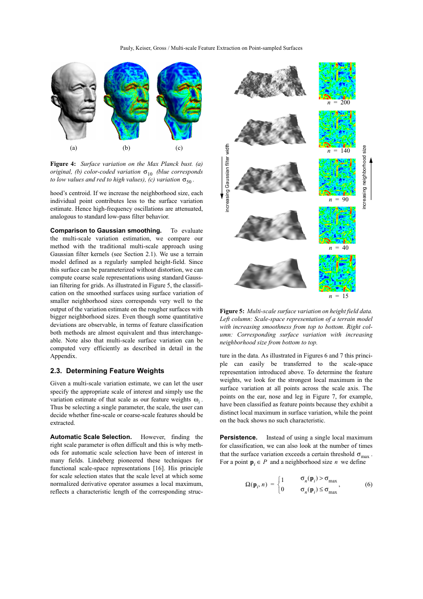
Figure 4: Surface variation on the Max Planck bust. (a)
original, (b) color-coded variation
(blue corresponds
to low values and red to high values), (c) variation
σ
σ
10
.
50
hood’s centroid. If we increase the neighborhood size, each
individual point contributes less to the surface variation
estimate. Hence high-frequency oscillations are attenuated,
analogous to standard low-pass filter behavior.
Comparison to Gaussian smoothing. To evaluate
the multi-scale variation estimation, we compare our
method with the traditional multi-scale approach using
Gaussian filter kernels (see Section 2.1). We use a terrain
model defined as a regularly sampled height-field. Since
this surface can be parameterized without distortion, we can
compute coarse scale representations using standard Gauss-
ian filtering for grids. As illustrated in Figure 5, the classifi-
cation on the smoothed surfaces using surface variation of
smaller neighborhood sizes corresponds very well to the
output of the variation estimate on the rougher surfaces with
bigger neighborhood sizes. Even though some quantitative
deviations are observable, in terms of feature classification
both methods are almost equivalent and thus interchange-
able. Note also that multi-scale surface variation can be
computed very efficiently as described in detail in the
Appendix.
2.3. Determining Feature Weights
Given a multi-scale variation estimate, we can let the user
specify the appropriate scale of interest and simply use the
variation estimate of that scale as our feature weights
.
i
Thus be selecting a single parameter, the scale, the user can
decide whether fine-scale or coarse-scale features should be
extracted.
ω
Automatic Scale Selection. However, finding
the
right scale parameter is often difficult and this is why meth-
ods for automatic scale selection have been of interest in
many fields. Lindeberg pioneered these techniques for
functional scale-space representations [16]. His principle
for scale selection states that the scale level at which some
normalized derivative operator assumes a local maximum,
reflects a characteristic length of the corresponding struc-
t
h
d
w
i
r
e
t
l
i
f
i
n
a
s
s
u
a
G
g
n
s
a
e
r
c
n
i
i
e
z
s
i
i
d
o
o
h
r
o
b
h
g
e
n
g
n
s
a
e
r
c
n
i
i
n
=
200
n
=
140
n
90=
n
40=
n
15=
Figure 5: Multi-scale surface variation on height field data.
Left column: Scale-space representation of a terrain model
with increasing smoothness from top to bottom. Right col-
umn: Corresponding surface variation with increasing
neighborhood size from bottom to top.
to
transferred
ture in the data. As illustrated in Figures 6 and 7 this princi-
ple can easily be
the scale-space
representation introduced above. To determine the feature
weights, we look for the strongest local maximum in the
surface variation at all points across the scale axis. The
points on the ear, nose and leg in Figure 7, for example,
have been classified as feature points because they exhibit a
distinct local maximum in surface variation, while the point
on the back shows no such characteristic.
Persistence. Instead of using a single local maximum
for classification, we can also look at the number of times
that the surface variation exceeds a certain threshold
.
For a point
and a neighborhood size
we define
max
σ
n
pi P∈
(
Ω pi n,
)
=
1
0
σ
σ
(
n pi
(
n pi
) σ
>
) σ
≤
,
max
max
(6)
�
Pauly, Keiser, Gross / Multi-scale Feature Extraction on Point-sampled Surfaces
σ
n
σ
n
σ
n
n
(a)
n
(b)
n
(c)
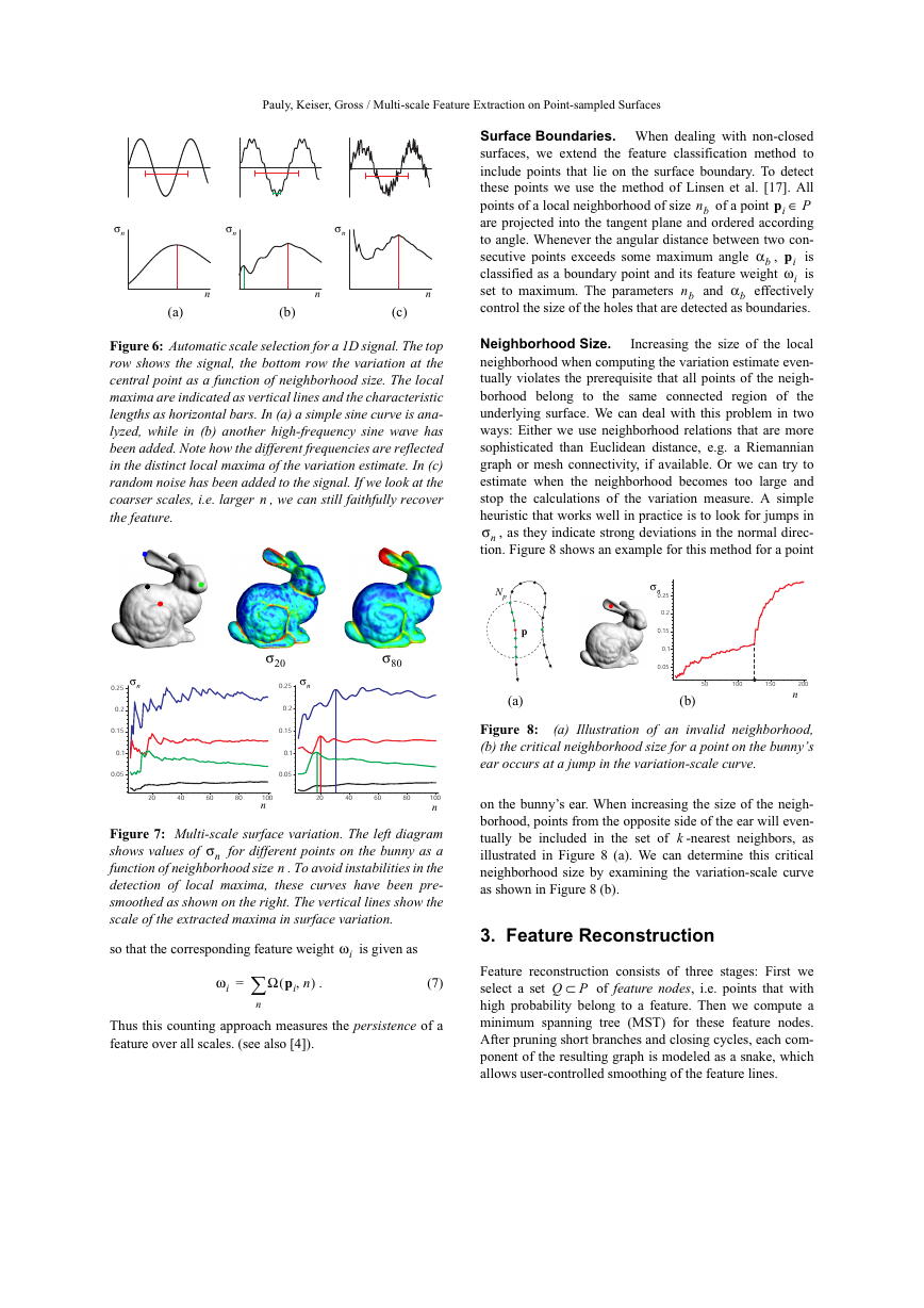
Figure 6: Automatic scale selection for a 1D signal. The top
row shows the signal, the bottom row the variation at the
central point as a function of neighborhood size. The local
maxima are indicated as vertical lines and the characteristic
lengths as horizontal bars. In (a) a simple sine curve is ana-
lyzed, while in (b) another high-frequency sine wave has
been added. Note how the different frequencies are reflected
in the distinct local maxima of the variation estimate. In (c)
random noise has been added to the signal. If we look at the
coarser scales, i.e. larger
, we can still faithfully recover
the feature.
n
σ
n
0.25
0.2
0.15
0.1
0.05
σ
80
σ
20
σ
n
0.25
0.2
0.15
0.1
0.05
20
40
60
80
100
n
20
40
60
80
100
n
n
σ
Figure 7: Multi-scale surface variation. The left diagram
for different points on the bunny as a
shows values of
function of neighborhood size
. To avoid instabilities in the
detection of local maxima, these curves have been pre-
smoothed as shown on the right. The vertical lines show the
scale of the extracted maxima in surface variation.
n
so that the corresponding feature weight
ω
i
is given as
ω
i
∑=
n
(
Ω pi n,
)
.
(7)
Thus this counting approach measures the persistence of a
feature over all scales. (see also [4]).
Surface Boundaries. When dealing with non-closed
surfaces, we extend the feature classification method to
include points that lie on the surface boundary. To detect
these points we use the method of Linsen et al. [17]. All
pi P∈
points of a local neighborhood of size
are projected into the tangent plane and ordered according
to angle. Whenever the angular distance between two con-
b piω
,
is
secutive points exceeds some maximum angle
classified as a boundary point and its feature weight
is
set to maximum. The parameters
effectively
control the size of the holes that are detected as boundaries.
of a point
and
nb
nb
i
α
α
b
Neighborhood Size. Increasing the size of the local
neighborhood when computing the variation estimate even-
tually violates the prerequisite that all points of the neigh-
borhood belong to the same connected region of the
underlying surface. We can deal with this problem in two
ways: Either we use neighborhood relations that are more
sophisticated than Euclidean distance, e.g. a Riemannian
graph or mesh connectivity, if available. Or we can try to
estimate when the neighborhood becomes too large and
stop the calculations of the variation measure. A simple
heuristic that works well in practice is to look for jumps in
σ
, as they indicate strong deviations in the normal direc-
tion. Figure 8 shows an example for this method for a point
n
Np
p
(a)
σ
n
0.25
0.2
0.15
0.1
0.05
50
100
150
200
n
(b)
Figure 8: (a) Illustration of an invalid neighborhood,
(b) the critical neighborhood size for a point on the bunny’s
ear occurs at a jump in the variation-scale curve.
on the bunny’s ear. When increasing the size of the neigh-
borhood, points from the opposite side of the ear will even-
tually be included in the set of
-nearest neighbors, as
illustrated in Figure 8 (a). We can determine this critical
neighborhood size by examining the variation-scale curve
as shown in Figure 8 (b).
k
3. Feature Reconstruction
Q P⊂
Feature reconstruction consists of three stages: First we
select a set
of feature nodes, i.e. points that with
high probability belong to a feature. Then we compute a
minimum spanning tree (MST) for these feature nodes.
After pruning short branches and closing cycles, each com-
ponent of the resulting graph is modeled as a snake, which
allows user-controlled smoothing of the feature lines.
�
Pauly, Keiser, Gross / Multi-scale Feature Extraction on Point-sampled Surfaces
3.1. Selecting feature nodes
i
i
pi P∈
to each sample point
In the classification stage of Section 2 we assigned weights
ω
that measure the confi-
pi
belongs to a feature. To select the relevant
dence that
Q P⊂
feature nodes
, we could discard all points whose
weights fall below a certain threshold. This hard threshold-
ing can cause undesirable artefacts, however, such as inter-
rupted or dangling feature lines. As suggested in [2],
hysteresis thresholding can alleviate these effects by using
<
. Points with corresponding
two thresholds
min
max
ω
weights smaller than
are discarded, while points with
ω
. All
will be used to bridge the
points with
gaps between feature nodes during the construction of the
minimum spanning tree (see below).
are included into the set of feature nodes
min
ω
≤
max
max
min
>
ω
ω
≤
ω
i
ω
ω
Q
3.2. Minimum spanning graph
To create a set of feature patterns we first compute the min-
imum spanning tree (MST) of the set of feature nodes
.
Q
qi Q⊂
according to
We start by ordering all feature nodes
their weights. Then we choose the feature node
with big-
gest weight as the seed point for the construction of the
MST. We define an edge for each of the
-nearest neigh-
bors
and compute corresponding edge cost as
of
q
q
k
qi
,(
c q qi
)
=
1
---------------
ω
ω
qi
q
γ
⋅+
q qi–
,
(8)
γ
where
is an additional parameter that allows us to balance
feature weights against Euclidean distance. All these edges
are put on a heap ordered by increasing cost values. Then
we take the edge with the smallest cost and add it to the
MST, if both edge nodes are not already part of the tree. For
the new feature node we compute a new set of edges and
corresponding cost values and also put these on the heap.
We repeat this process until the heap is empty. Figure 9 (b)
shows the MST of the dinosaur head generated with this
algorithm.
Pruning and closing cycles. As can be seen in this
example, the MST of all feature nodes contains many short
branches, which are usually treated as artefacts that do not
describe salient features. To eliminate these short branches
from our set of feature patterns, we use a bottom up graph
pruning method. Our algorithm starts by sorting all leaves
of the MST according to their depth. By traversing the tree
upward from the deepest node, we can determine the long-
est path, which defines a new root of the MST. Now we
recursively compute all branches of the tree and assign to
each branch an importance value that is given as the length
of the branch multiplied by the product of all edge weights.
Thus we retain short branches that contain feature nodes
with high confidence values and only prune those branches
that with low probability are part of a feature line.
The MST construction above does not support cycles in
the feature lines. It is often desirable, however, to allow
closed loops as these more naturally describe certain feature
lines. Therefore we transform the MST into a graph by clos-
ing cycles that are longer than a user-specified threshold. To
close a cycle, we use those edges whose feature nodes are
already in the graph. From both these nodes we traverse the
tree upward until the two paths cross at a common node.
The sum of the two path lengths then equals the cycle
length. Note that our method for pruning and closing cycles
does not require an expensive breadth first search as was
done, for example, in [5]. Figure 9 (c) shows the MST of
Figure 9 (b) after pruning and closing cycles.
(a)
(c)
(b)
(d)
Figure 9: Feature reconstruction on the dinosaur head: (a)
feature weights, (b) minimum spanning tree of feature
nodes, (c) MST after pruning and closing cycles, (d) smooth-
ing with snakes.
3.3. Active Contour Models
As can be seen in Figure 9 (c), the extracted feature lines
connect samples of the original point cloud and are often
jagged. This might be acceptable for partitioning algo-
rithms, but for feature-based visualization methods (see
Section 4) it leads to inferior rendering quality. We there-
fore need a mechanism for smoothing feature lines. Spline
fitting has been used in previous approaches [5], but we
found that it does not provide enough flexibility and control
over the smoothness and accuracy of the extracted feature
lines. In [11], Kass et al. introduced snakes, active contour
models, for detecting features in images. A snake is an
energy-minimizing spline that moves under internal and
external forces. We use snakes to smooth the feature curves,
while maintaining a close contact to the surface. The main
benefit of snakes is their explicit control over the degree of
�
Pauly, Keiser, Gross / Multi-scale Feature Extraction on Point-sampled Surfaces
smoothness that can be adapted to the specific application
needs. Additionally, external constraints can easily be
incorporated, for instance to enable user interaction for
positioning feature lines.
Energy Minimization. We model each component of
the MSG as a parametric curve
that tries to minimize
the energy functional
v s( )
E
∫=
Eint v s( )
(
) Eext v s( )
+
(
)
sd
,
(9)
The internal spline energy consists of first- and second-
order terms, modeling the behavior of a membrane and a
thin plate, respectively:
⋅
v s( )′ 2 β s( ) v s( )″ 2 2⁄
+
⋅
,
(10)
)
=
(
Eint v s( )
α s( )
α s( )
β s( )
and
where
control the relative weight of the two
terms. The external energy is related to the surface varia-
tion:
(
)
,
)
(
=
(11)
(
σ˜ v s( )
⁄
1 σ˜ v s( )
Eext v s( )
)
is computed by interpolating the maximum
where
. Discretization of the
variation of each point
functional
finally leads to a system of Euler equations
that we solve using Euler integration (see [11] for details).
Figure 9 (d) shows the smoothing effect on the dinosaur
head.
p P∈
v s( )
at
E
4. Non-photorealistic Rendering
The feature lines extracted by our method can be used as
input for a variety of processing algorithms, including mesh
generation, anisotropic fairing and model segmentation. In
this section we introduce a point rendering system for creat-
ing line drawings of point-sampled surfaces. Based on the
surface splatting technique of Zwicker et. al. [25], our ren-
derer takes as input a surfel model of the original surface
and the output of our feature extraction method. Each fea-
ture line is converted into a set of feature surfels by sam-
pling the model surface along the feature line. The surfels
of the original model are only rendered into the z-buffer to
resolve visibility and are assigned the background color.
The final image is then only composed of the visible feature
surfels. Note that no shading computations are applied,
which significantly improves rendering performance.
To enhance the semantics of our renditions, we can uti-
lize the additional information of the classification stage.
We scale the splat radii of the feature surfels according to
scale and adjust the intensity (e.g. grey level) according to
the maximum surface variation. Thus features on coarser
scales are rendered as thicker lines, while features on fine
scales are rendered as thinner lines. Also prominent features
are rendered at high intensities, while less significant fea-
tures are rendered at low intensity. With these simple exten-
sions, we achieve a very intuitive effect, similar to what an
painter would do when drawing an image. To obtain more
artistic looking renditions, we apply an additional screen
space filter, as illustrated in Figures 10 to 14.
5. Results
We have implemented the feature extraction pipeline
described in the previous sections and tested our method on
a variety of point-sampled surfaces. Tables 1 and 2 summa-
rize performance data for the different stages of the pipe-
line. For multi-scale classification we evaluate the surface
variation estimate
for all neigh-
borhood sizes
between 15 and 200 using the method
described in the Appendix. We use kd-trees for computing
the set of
-nearest neighbors, similar to [19]. Note that the
interactive feedback loop for adjusting the various thresh-
olding parameters does not include the multi-scale classifi-
cation stage, which hence needs to be executed only once.
for each point
p P∈
σ
n
k
n
Model
Igea
Cat
Gnome
Dinosaur
Dragon
multi-scale-
classification
MST, pruning,
closing cycles
snakes (100 Eul-
er steps)
25.156
1.829
6.703
10.187
64.422
1.468
0.062
0.203
2.484
8.469
0.203
0.031
0.047
0.234
1.125
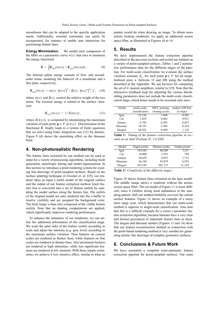
Table 1: Timing of the feature extraction pipeline in sec-
onds on an Intel Pentium IV, 2.8 GHz.
Model
Igea
Cat
Gnome
Dinosaur
Dragon
#input points
134,345
10,000
54,659
56,194
435,545
#feature nodes
40,509
3,593
9,655
45,879
203,713
#snake points
7,327
798
1,714
6,395
31,154
Table 2: Complexity of the different stages.
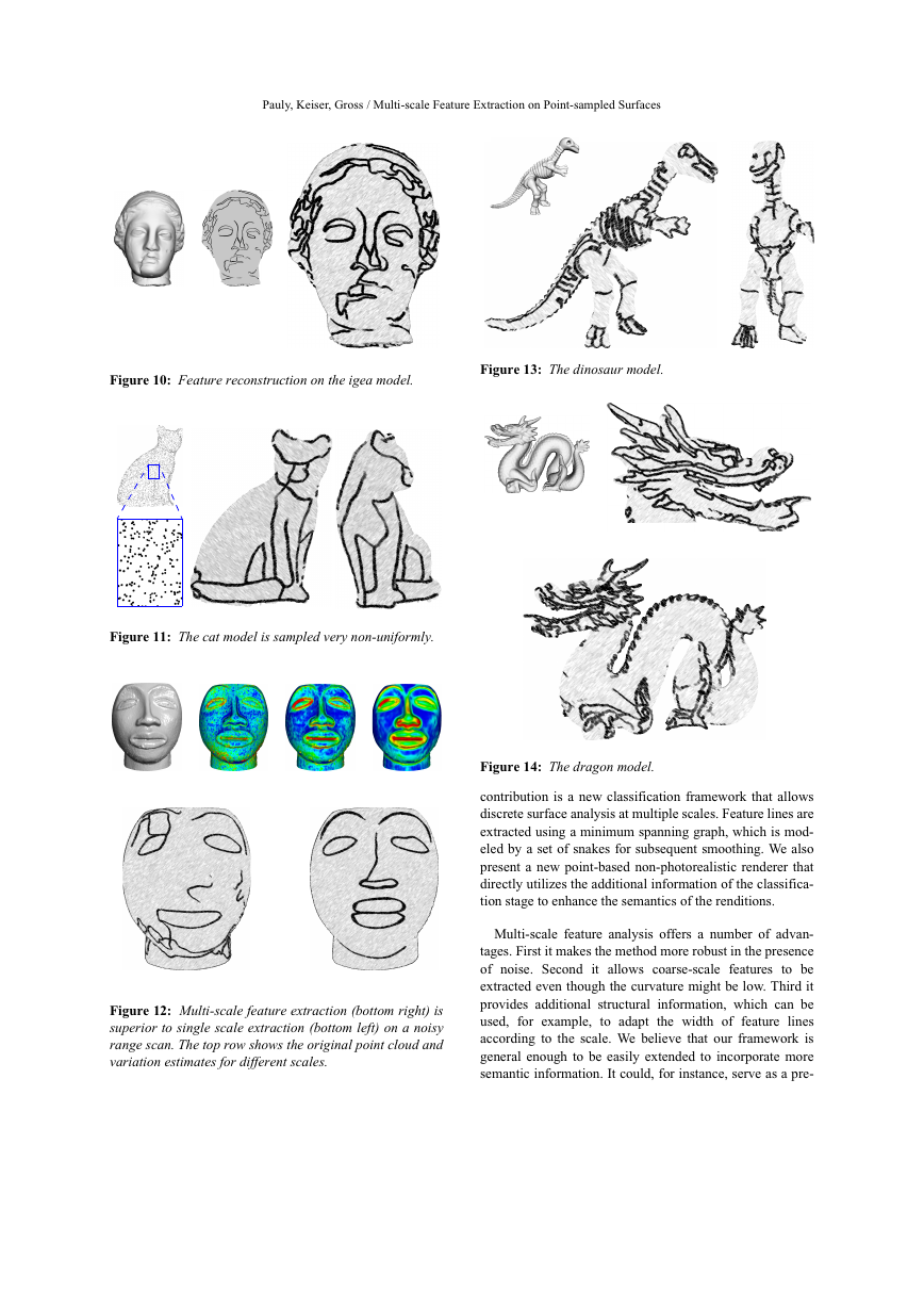
Figure 10 shows feature lines extracted on the Igea model.
The middle image shows a rendition without the artistic
screen space filter. The cat model of Figure 11 is more diffi-
cult, since it exhibits strong local imbalances in the sam-
pling pattern. Still our method faithfully recovers the salient
surface features. Figure 12 shows an example of a noisy
laser range scan, which demonstrates that our multi-scale
method is superior to single-scale classification. Also note
that this is a difficult example for a (semi-) automatic fea-
ture extraction algorithm, because humans have a very clear
and distinct perception of important feature lines in faces.
The dragon and dinosaur models (Figures 13 and 14) show
that our feature reconstruction method in connection with
the point-based rendering method is very suitable for gener-
ating artistic line drawings of complex geometric surfaces.
6. Conclusions & Future Work
We have presented a complete semi-automatic feature
extraction pipeline for point-sampled surfaces. Our main
�
Pauly, Keiser, Gross / Multi-scale Feature Extraction on Point-sampled Surfaces
Figure 10: Feature reconstruction on the igea model.
Figure 13: The dinosaur model.
Figure 11: The cat model is sampled very non-uniformly.
Figure 14: The dragon model.
contribution is a new classification framework that allows
discrete surface analysis at multiple scales. Feature lines are
extracted using a minimum spanning graph, which is mod-
eled by a set of snakes for subsequent smoothing. We also
present a new point-based non-photorealistic renderer that
directly utilizes the additional information of the classifica-
tion stage to enhance the semantics of the renditions.
Multi-scale feature analysis offers a number of advan-
tages. First it makes the method more robust in the presence
of noise. Second it allows coarse-scale features to be
extracted even though the curvature might be low. Third it
provides additional structural information, which can be
used, for example, to adapt the width of feature lines
according to the scale. We believe that our framework is
general enough to be easily extended to incorporate more
semantic information. It could, for instance, serve as a pre-
Figure 12: Multi-scale feature extraction (bottom right) is
superior to single scale extraction (bottom left) on a noisy
range scan. The top row shows the original point cloud and
variation estimates for different scales.
�




 2023年江西萍乡中考道德与法治真题及答案.doc
 2012年重庆南川中考生物真题及答案.doc
 2013年江西师范大学地理学综合及文艺理论基础考研真题.doc
 2020年四川甘孜小升初语文真题及答案I卷.doc
 2020年注册岩土工程师专业基础考试真题及答案.doc
 2023-2024学年福建省厦门市九年级上学期数学月考试题及答案.doc
 2021-2022学年辽宁省沈阳市大东区九年级上学期语文期末试题及答案.doc
 2022-2023学年北京东城区初三第一学期物理期末试卷及答案.doc
 2018上半年江西教师资格初中地理学科知识与教学能力真题及答案.doc
 2012年河北国家公务员申论考试真题及答案-省级.doc
 2020-2021学年江苏省扬州市江都区邵樊片九年级上学期数学第一次质量检测试题及答案.doc
 2022下半年黑龙江教师资格证中学综合素质真题及答案.doc