This article has been accepted for inclusion in a future issue of this journal. Content is final as presented, with the exception of pagination.
IEEE TRANSACTIONS ON NEURAL NETWORKS AND LEARNING SYSTEMS
1
Broad Learning System: An Effective and Efficient
Incremental Learning System Without
the Need for Deep Architecture
C. L. Philip Chen, Fellow, IEEE, and Zhulin Liu
Abstract— Broad Learning System (BLS) that aims to offer
an alternative way of learning in deep structure is proposed
in this paper. Deep structure and learning suffer from a time-
consuming training process because of a large number of con-
necting parameters in filters and layers. Moreover, it encounters
a complete retraining process if the structure is not sufficient to
model the system. The BLS is established in the form of a flat
network, where the original inputs are transferred and placed as
“mapped features” in feature nodes and the structure is expanded
in wide sense in the “enhancement nodes.” The incremental
learning algorithms are developed for fast remodeling in broad
expansion without a retraining process if the network deems
to be expanded. Two incremental learning algorithms are given
for both the increment of the feature nodes (or filters in deep
structure) and the increment of the enhancement nodes. The
designed model and algorithms are very versatile for selecting
a model rapidly. In addition, another incremental learning is
developed for a system that has been modeled encounters a new
incoming input. Specifically, the system can be remodeled in an
incremental way without the entire retraining from the beginning.
Satisfactory result for model reduction using singular value
decomposition is conducted to simplify the final structure. Com-
pared with existing deep neural networks, experimental results
on the Modified National Institute of Standards and Technology
database and NYU NORB object recognition dataset benchmark
data demonstrate the effectiveness of the proposed BLS.
Index Terms— Big data, big data modeling, broad learning
system (BLS), deep learning,
learning, random
vector functional-link neural networks (RVFLNN), single layer
feedforward neural networks (SLFN), singular value decomposi-
tion (SVD).
incremental
I. INTRODUCTION
D EEP structure neural networks and learnings have been
applied in many fields and have achieved breakthrough
successes in a great number of applications [1], [2], partic-
ularly in large scale data processing [3], [4]. Among them,
Manuscript received March 25, 2017; revised May 20, 2017 and June 11,
2017; accepted June 12, 2017. This work was supported in part by Macao
Science and Technology Development Fund under Grant 019/2015/A1, in
part by UM Research Grants, and in part by the National Nature Sci-
ence Foundation of China under Grant 61572540. (Corresponding author:
C. L. Philip Chen.)
C. L. P. Chen is with the Department of Computer and Information Science,
Faculty of Science and Technology, University of Macau, Macau 99999,
China; with Dalian Maritime University, Dalian 116026, China; and also with
the State Key Laboratory of Management and Control for Complex Systems,
Institute of Automation, Chinese Academy of Sciences, Beijing 100080, China
(e-mail: philip.chen@ieee.org).
Z. Liu is with the Department of Computer and Information Science,
Faculty of Science and Technology, University of Macau, Macau 99999, China
(e-mail: zhulinlau@gmail.com).
Color versions of one or more of the figures in this paper are available
online at http://ieeexplore.ieee.org.
Digital Object Identifier 10.1109/TNNLS.2017.2716952
the most popular deep networks are the deep belief networks
(DBN) [5], [6], the deep Boltzmann machines (DBM) [7], and
the convolutional neural networks (CNN) [8], [9]. Although
the deep structure has been so powerful, most of networks
suffer from the time-consuming training process because
a great number of hyperparameters and complicated struc-
tures are involved. Moreover,
this complication makes it
so difficult to analyze the deep structure theoretically that
most work span in turning the parameters or stacking more
layers for better accuracy. To achieve this mission, more
and more powerful computing resource has been involved.
Recently, some variations in hierarchical structure [10]–[12] or
ensembles [13]–[17], are proposed to improve the training
performance.
Single layer feedforward neural networks (SLFN) have been
widely applied to solve problems such as classification and
regression because of their universal approximation capabil-
ity [18]–[21]. Conventional methods for training SLFN are
gradient-descent-based learning algorithms [22], [23]. The
generalization performance of them is more sensitive to the
parameter settings such as learning rate. Similarly, they usually
suffer from slow convergence and trap in a local minimum.
The random vector functional-link neural network (RVFLNN),
proposed in [19]–[21], offers a different learning method.
RVFLNN effectively eliminates the drawback of the long
training process and also it provides the generalization capa-
bility in function approximation [20], [24]. It has been proven
that RVFLNN is a universal approximation for continuous
functions on compact sets with fast learning property. There-
fore, RVFLNN has been employed to solve problems in
diverse domains, including the context of modeling and con-
trol [25]. Although RVFLNN enhances the performance of the
perception significantly, this technique could not work well
on remodeling high-volume and time-variety data in modern
large data era [26]. To model moderate data size, a dynamic
step-wise updating algorithm was proposed in [27] to update
the output weights of the RVFLNN for both a new added
pattern and a new added enhancement node. This paper paves
a path for remodeling the system that has been modeled and
encounters a new incoming data.
Nowadays, in addition to the growth of data in size, the
data dimensions also increase tremendously. Taking the raw
data with high dimension directly to a neural network, the
system cannot sustain its accessibility anymore. The challenge
for solving high dimensional data problem becomes imperative
recently. Two common practices to alleviate this problem are
dimension reduction and feature extraction. Feature extraction
2162-237X © 2017 IEEE. Personal use is permitted, but republication/redistribution requires IEEE permission.
See http://www.ieee.org/publications_standards/publications/rights/index.html for more information.
�
This article has been accepted for inclusion in a future issue of this journal. Content is final as presented, with the exception of pagination.
2
IEEE TRANSACTIONS ON NEURAL NETWORKS AND LEARNING SYSTEMS
is to seek, possible, the optimal transformation from the input
data into the feature vectors. Common approaches, which
have the advantage of easy implementation and outstanding
efficiency, for feature selection include variable ranking [28],
feature subset selection [29], penalized least squares [30],
random feature extractions such as nonadaptive random pro-
jections [31] and random forest [32], or convolution-based
input mapping, to name a few.
Likewise for the feature extraction, the RVFLNN can take
mapped features as its input. The proposed Broad Learning
System (BLS) is designed based on the idea of RVFLNN.
In addition, the BLS can effectively and efficiently update the
systems (or relearn) incrementally when it deems necessary.
The BLS is designed as, first, the mapped features are gener-
ated from the input data to form the feature nodes. Second, the
mapped features are enhanced as enhancement nodes with ran-
domly generated weights. The connections of all the mapped
features and the enhancement nodes are fed into the output.
Ridge regression of the pseudoinverse is designed to find
the desired connection weights. Broad Learning algorithms
are designed for the network through the broad expansion
in both the feature nodes and the enhancement nodes. And
the incremental learning algorithms are developed for fast
remodeling in broad expansion without a retraining process
if the network deems to be expanded.
It should be noted that once the learning system has com-
pleted its modeling, it may consist of some redundancy due to
the broad expansion. The system can be simplified more using
low-rank approximations. Low-rank approximation has been
established as a new tool in scientific computing to address
large-scale linear and multilinear algebra problems, which
would be intractable by classical techniques. In [33] and [34],
comprehensive exposition of the theory, algorithms, and appli-
cations of structured low-rank approximations are presented.
Among the various algorithms, the singular value decomposi-
tion (SVD) and nonnegative matrix factorization (NMF) [35]
are widely used for exploratory data analysis. By embedding
these classical low-rank algorithms into the proposed broad
learning network, we also design an SVD-based structure to
simplify broad learning algorithm. This simplification process
can be done by compressing the system on-the-fly right after
the moment when additional feature nodes are inserted or right
after additional enhancement nodes are inserted or after both
together. One can also choose to compress the whole structure
after the learning is completed. The algorithms are designed so
versatile such that one can select number of equivalent neural
nodes in the final structure. This approach lays out an excellent
approach for model selection.
This paper is organized as follows. In Section II, prelimi-
naries of RVFLNN, ridge regression approach of pseudoin-
verse, sparse autoencoder, and SVD are given. Section III
presents the BLS and gives the details of the proposed broad
learning algorithms. Section IV compares the performance
in Modified National Institute of Standards and Technology
database (MNIST) classification and NYU object recognition
benchmark (NORB) classification with those from various
deep systems. Also the performance analysis of the proposal
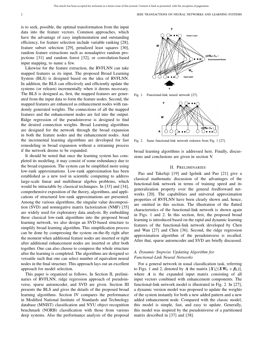
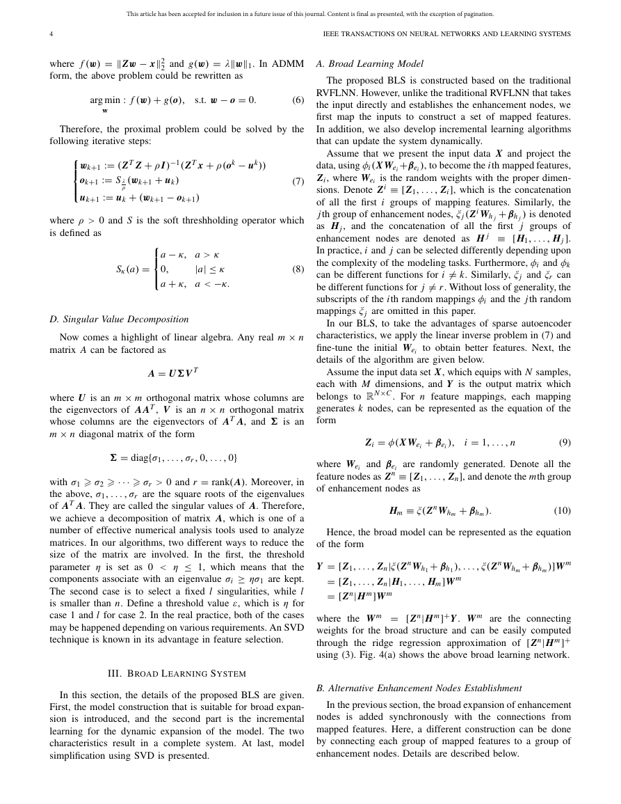
Fig. 1. Functional-link neural network [27].
Fig. 2. Same functional-link network redrawn from Fig. 1 [27].
broad learning algorithms is addressed here. Finally, discus-
sions and conclusions are given in section V.
II. PRELIMINARIES
Pao and Takefuji [19] and Igelnik and Pao [21] give a
classical mathematic discussion of the advantages of the
functional-link network in terms of training speed and its
generalization property over the general feedforward net-
works [20]. The capabilities and universal approximation
properties of RVFLNN have been clearly shown and, hence,
are omitted in this section. The illustration of the flatted
characteristics of the functional-link network is shown again
in Figs. 1 and 2. In this section, first, the proposed broad
learning is introduced based on the rapid and dynamic learning
features of the functional-link network developed by Chen
and Wan [27] and Chen [36]. Second, the ridge regression
approximation algorithm of the pesudoinverse is recalled.
After that, sparse autoencoder and SVD are briefly discussed.
A. Dynamic Stepwise Updating Algorithm for
Functional-Link Neural Networks
For a general network in usual classification task, referring
to Figs. 1 and 2, denoted by A the matrix [X|ξ(X Wh + βh )],
where A is the expanded input matrix consisting of all
input vectors combined with enhancement components. The
functional-link network model is illustrated in Fig. 2. In [27],
a dynamic version model was proposed to update the weights
of the system instantly for both a new added pattern and a new
added enhancement node. Compared with the classic model,
this model is simple, fast, and easy to update. Generally,
this model was inspired by the pseudoinverse of a partitioned
matrix described in [37] and [38].
�
This article has been accepted for inclusion in a future issue of this journal. Content is final as presented, with the exception of pagination.
CHEN AND LIU: BLS: AN EFFECTIVE AND EFFICIENT INCREMENTAL LEARNING SYSTEM
3
Fig. 3.
Illustration of stepwise update algorithm [27].
Denote An be the n × m pattern matrix. In this section, we
will only introduce the stepwise updating algorithm for adding
a new enhancement node to the network as shown in Fig. 3.
In this case, it is equivalent to add a new column to the input
matrix An. Denote An+1 [ An|a]. Then the pseudoinverse
+
n+1 equals
of the new A
+
A
n
− d bT
bT
where d = A
+
n a
bT =
and c = a − And.
Again, the new weights are
(c)+
(1 + d T d)−1d T A
+
n
Wn+1 =
Wn − d bT Yn
bT Yn
if c = 0
if c = 0
where Wn+1 and Wn are the weights after and before new
enhancement nodes are added, respectively. In this way, the
new weights can be updated easily by only computing the
pseudoinverse of the corresponding added node. It should be
noted that if An is of the full rank, then c = 0 which will make
+
a fast updating of the pseudoinverse A
n and the weight Wn.
B. Pseudoinverse and Ridge Regression Learning Algorithms
In a flatted network, pseudoinverse can be considered as
a very convenient approach to solve the output-layer weights
of a neural network. Different methods can be used to cal-
culate this generalized inverse, such as orthogonal projec-
tion method, orthogonalization method, iterative method, and
SVD [39], [40]. However, a direct solution is too expensive,
especially the training samples and input patterns are suffered
from high volume, high velocity, and/or high variety [26].
Also, pseudoinverse, which is the least square estimator of
linear equations, is aimed to reach the output weights with the
smallest training errors, but may not true for generalization
errors, especially for the ill condition problems. In fact, the
following kind of optimal problems is an alternative way to
solve the pseudoinverse:
: AW − Yσ1
v + λWσ2
u
arg min
W
(1)
where σ1 > 0, σ2 > 0, and u, v are typically kinds of norm
regularization. By taking σ1 = σ2 = u = v = 2, the above
optimal problem is setting as regular l2 norm regularization,
which is convex and has a better generalization performance.
The value λ denotes the further constraints on the sum of the
squared weights, W. This solution is equivalent with the
ridge regression theory, which gives an approximation to
the Moore−Penrose generalized inverse by adding a positive
number to the diagonal of AT A or A AT [41]. Theoretically,
if λ = 0, the inverse problem degenerates into the least square
problem and leads the solution to original pesuedoinverse.
On the other hand,
the solution is heavily
constrained and tends to 0. Consequently, we have
if λ → ∞,
W = (λI + A AT )−1 AT Y .
Specifically, we have that
+ = lim
A
λ→0
(λI + A AT )−1 AT .
(2)
(3)
C. Sparse Autoencoder
Supervised learning tasks, such as classifications, usually
need a good feature representation of the input to achieve
an outstanding performance. Feature representation is not
only an efficient way of data representation, but also, more
importantly, it captures the characteristics of the data. Usually,
intractable mathematic derivation is used or an easy random
initialization to generate a set of random features can be
populated. However, randomness suffers from unpredictability
and needs guidance. To overcome the randomness nature,
the sparse autoencoder could be regarded as an important
tool to slightly fine-tune the random features to a set of
sparse and compact features. Specifically, sparse feature learn-
ing models have been attractive that could explore essential
characterization [12], [42], [43].
To extract the sparse features from the given training data,
X can be considered to solve the optimization problem [44].
Notice that it is equivalent to the optimization problem in (1)
if we set σ2 = u = 1, and σ1 = v = 2
: Z ˆW − X2
+ λ ˆW1
(4)
2
arg minˆW
ˆW is the sparse autoencoder solution and Z is the
where
desired output of the given linear equation, i.e., X W = Z.
The above problem denoted by lasso in [45] is con-
vex. Consequently, the approximation problem in (4) can be
solved by dozens of ways, such as orthogonal matching pur-
suit [46], K-SVD [47], alternating direction method of multi-
pliers (ADMM) [48], and fast iterative shrinkage-thresholding
algorithm (FISTA) [49]. Among them, the ADMM method
is actually designed for general decomposition methods and
decentralized algorithms in the optimization problems. More-
over, it has been shown that many state-of-art algorithms for
l1 norm involved problems could be derived by ADMM [50],
such as FISTA. Hence, a brief review of typical approach for
lasso is presented below.
First, (4) can be equivalently considered as the following
general problem:
: f (w) + g(w), w ∈ Rn
(5)
arg min
w
�
This article has been accepted for inclusion in a future issue of this journal. Content is final as presented, with the exception of pagination.
4
IEEE TRANSACTIONS ON NEURAL NETWORKS AND LEARNING SYSTEMS
where f (w) = Zw − x2
form, the above problem could be rewritten as
2 and g(w) = λw1. In ADMM
: f (w) + g(o),
s.t. w − o = 0.
(6)
arg min
w
Therefore, the proximal problem could be solved by the
following iterative steps:
wk+1 := (ZT Z + ρ I)−1(ZT x + ρ(ok − uk))
ok+1 := S λ
uk+1 := uk + (wk+1 − ok+1)
(wk+1 + uk)
ρ
(7)
⎧⎪⎨
⎪⎩
where ρ > 0 and S is the soft threshholding operator which
is defined as
⎧⎪⎨
⎪⎩
Sκ (a) =
a − κ, a > κ
|a| ≤ κ
0,
a + κ, a < −κ.
(8)
D. Singular Value Decomposition
Now comes a highlight of linear algebra. Any real m × n
matrix A can be factored as
A = U�V T
where U is an m × m orthogonal matrix whose columns are
the eigenvectors of A AT , V is an n × n orthogonal matrix
whose columns are the eigenvectors of AT A, and � is an
m × n diagonal matrix of the form
� = diag{σ1, . . . , σr , 0, . . . , 0}
with σ1 σ2 ··· σr > 0 and r = rank( A). Moreover, in
the above, σ1, . . . , σr are the square roots of the eigenvalues
of AT A. They are called the singular values of A. Therefore,
we achieve a decomposition of matrix A, which is one of a
number of effective numerical analysis tools used to analyze
matrices. In our algorithms, two different ways to reduce the
size of the matrix are involved. In the first, the threshold
parameter η is set as 0 < η ≤ 1, which means that the
components associate with an eigenvalue σi ≥ ησ1 are kept.
The second case is to select a fixed l singularities, while l
is smaller than n. Define a threshold value ε, which is η for
case 1 and l for case 2. In the real practice, both of the cases
may be happened depending on various requirements. An SVD
technique is known in its advantage in feature selection.
A. Broad Learning Model
The proposed BLS is constructed based on the traditional
RVFLNN. However, unlike the traditional RVFLNN that takes
the input directly and establishes the enhancement nodes, we
first map the inputs to construct a set of mapped features.
In addition, we also develop incremental learning algorithms
that can update the system dynamically.
+βei
Assume that we present the input data X and project the
data, using φi (X Wei
), to become the ith mapped features,
Zi, where Wei is the random weights with the proper dimen-
sions. Denote Zi ≡ [Z1, . . . , Zi], which is the concatenation
of all the first i groups of mapping features. Similarly, the
+ βh j
jth group of enhancement nodes, ξ j (Zi Wh j
) is denoted
as Hj , and the concatenation of all the first
j groups of
enhancement nodes are denoted as H j ≡ [H1, . . . , Hj].
In practice, i and j can be selected differently depending upon
the complexity of the modeling tasks. Furthermore, φi and φk
can be different functions for i = k. Similarly, ξ j and ξr can
be different functions for j = r. Without loss of generality, the
subscripts of the ith random mappings φi and the jth random
mappings ξ j are omitted in this paper.
In our BLS, to take the advantages of sparse autoencoder
characteristics, we apply the linear inverse problem in (7) and
fine-tune the initial Wei
to obtain better features. Next, the
details of the algorithm are given below.
Assume the input data set X, which equips with N samples,
each with M dimensions, and Y is the output matrix which
belongs to RN×C . For n feature mappings, each mapping
generates k nodes, can be represented as the equation of the
form
Zi = φ(X Wei
+ βei
),
i = 1, . . . , n
(9)
where Wei and βei are randomly generated. Denote all the
feature nodes as Zn ≡ [Z1, . . . , Zn], and denote the mth group
of enhancement nodes as
Hm ≡ ξ(ZnWhm
+ βhm
).
(10)
Hence, the broad model can be represented as the equation
of the form
Y = [Z1, . . . , Zn|ξ(ZnWh1
+ βh1
= [Z1, . . . , Zn|H1, . . . , Hm]W m
= [Zn|Hm]W m
), . . . , ξ(ZnWhm
+ βhm
)]W m
where the W m = [Zn|Hm]+
Y . W m are the connecting
weights for the broad structure and can be easily computed
through the ridge regression approximation of [Zn|Hm]+
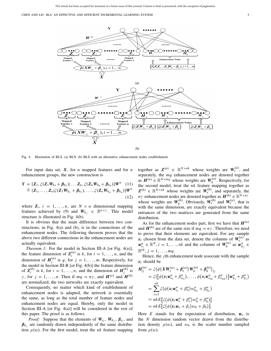
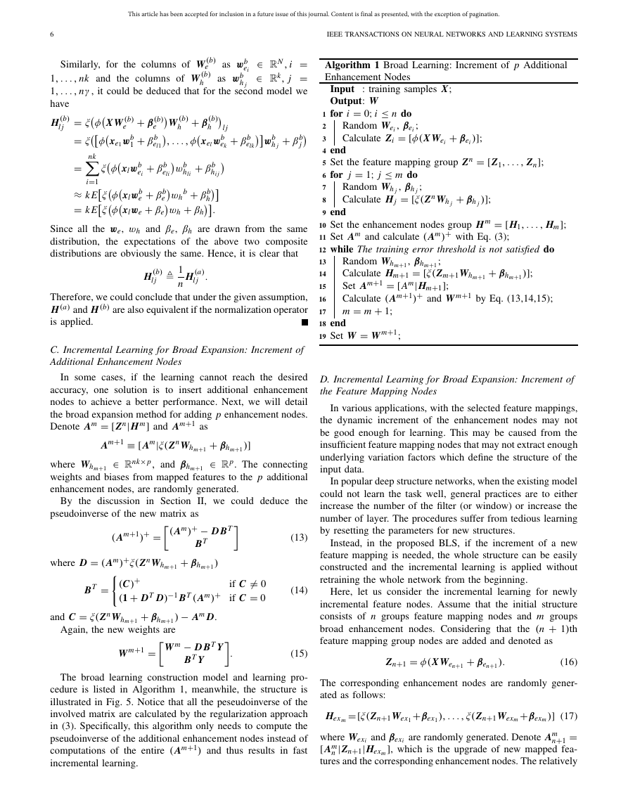
using (3). Fig. 4(a) shows the above broad learning network.
III. BROAD LEARNING SYSTEM
In this section, the details of the proposed BLS are given.
First, the model construction that is suitable for broad expan-
sion is introduced, and the second part is the incremental
learning for the dynamic expansion of the model. The two
characteristics result in a complete system. At last, model
simplification using SVD is presented.
B. Alternative Enhancement Nodes Establishment
In the previous section, the broad expansion of enhancement
nodes is added synchronously with the connections from
mapped features. Here, a different construction can be done
by connecting each group of mapped features to a group of
enhancement nodes. Details are described below.
�
This article has been accepted for inclusion in a future issue of this journal. Content is final as presented, with the exception of pagination.
CHEN AND LIU: BLS: AN EFFECTIVE AND EFFICIENT INCREMENTAL LEARNING SYSTEM
5
Fig. 4.
Illustration of BLS. (a) BLS. (b) BLS with an alternative enhancement nodes establishment.
For input data set, X, for n mapped features and for n
enhancement groups, the new construction is
)| . . . Zn, ξ(ZnWhn
+ βh1
+ βhn
), . . . , ξ(ZnWhn
Y = [Z1, ξ(Z1Wh1
+ βh1
[Z1, . . . , Zn|ξ(Z1Wh1
(11)
)]W n
(12)
where Zi , i = 1, . . . , n, are N × α dimensional mapping
α×γ . This model
features achieved by (9) and Wh j
structure is illustrated in Fig. 4(b).
)]W n
+ βhn
∈ R
It is obvious that the main difference between two con-
structions, in Fig. 4(a) and (b), is in the connections of the
enhancement nodes. The following theorem proves that the
above two different connections in the enhancement nodes are
actually equivalent.
i
Theorem 1: For the model in Section III-A [or Fig. 4(a)],
is k, for i = 1, . . . , n, and the
the feature dimension of Z(a)
is q, for j = 1, . . . , m. Respectively, for
dimension of H (a)
the model in Section III-B [or Fig. 4(b)] the feature dimension
of Z(b)
is
γ , for j = 1, . . . , n. Then if mq = nγ , and H (a) and H (b)
are normalized, the two networks are exactly equivalent.
is k, for i = 1, . . . , n, and the dimension of H (b)
j
i
j
Consequently, no matter which kind of establishment of
enhancement nodes is adapted,
the network is essentially
the same, as long as the total number of feature nodes and
enhancement nodes are equal. Hereby, only the model in
Section III-A [or Fig. 4(a)] will be considered in the rest of
this paper. The proof is as follows.
Proof: Suppose that the elements of Wei , Wh j , βei , and
βh j are randomly drawn independently of the same distribu-
tion ρ(w). For the first model, treat the nk feature mapping
e
e
h
together as Z(a) ∈ RN×nk whose weights are W (a)
, and
separately, the mq enhancement nodes are denoted together
as H (a) ∈ RN×mq whose weights are W (a)
. Respectively, for
the second model, treat the nk feature mapping together as
Z(b) ∈ RN×nk whose weights are W (b)
, and separately, the
nγ enhancement nodes are denoted together as H (b) ∈ RN×nγ
whose weights are W (b)
h . Obviously, W (b)
, that is
with the same dimension, are exactly equivalent because the
entrances of the two matrices are generated from the same
distribution.
As for the enhancement nodes part, first we have that H (a)
and H (b) are of the same size if mq = nγ . Therefore, we need
to prove that their elements are equivalent. For any sample
xl chosen from the data set, denote the columns of W (a)
as
∈
e
as wa
wa
Rnk, j = 1, . . . , mq.
ei
h j
Hence, the jth enhancement node associate with the sample
∈ RN , i = 1, . . . , nk and the columns of W (a)
and W (a)
h
e
e
l j
+ βa
elnk
e
h
φ
xl should be
= ξ
H (a)
X W (a)
φ
e
l j
= ξ
xlwa
= nk
e1
i=1
≈ nk E
= nk E
φ
φ
φ
ξ
el1
+ β(a)
+ βa
W (a)
, . . . , φ
+ β(a)
h
xlwa
enk
+ βa
+ βa
+ βa
+ βa
xlwa
wa
e
h
wh + βh
xlwe + βe
wa
hli
xlwa
ei
hli
li
ξ
ξ
h
e
.
wa
h j
+ βa
h j
Here E stands for the expectation of distribution, we is
the N dimension random vector drawn from the distribu-
tion density ρ(w), and wh is the scaler number sampled
from ρ(w).
�
This article has been accepted for inclusion in a future issue of this journal. Content is final as presented, with the exception of pagination.
6
IEEE TRANSACTIONS ON NEURAL NETWORKS AND LEARNING SYSTEMS
∈ RN , i =
Similarly, for the columns of W (b)
e
∈ Rk, j =
1, . . . , nk and the columns of W (b)
h
1, . . . , nγ , it could be deduced that for the second model we
have
H (b)
l j
as wb
ei
as wb
h j
φ
e
+ βb
elk
+ βb
j
wb
h j
φ
= ξ
= ξ
= nk
i=1
≈ k E
= k E
+ β(b)
+ βb
X W (b)
e
wb
xe1
1
xlwb
ei
W (b)
h
, . . . , φ
+ β(b)
h
l j
wb
xel
ek
+ βb
+ βb
wb
hli
b + βb
+ βb
xlwb
wh
e
wh + βh
xlwe + βe
hi j
el1
eli
φ
φ
φ
ξ
h
ξ
ξ
e
.
Since all the we, wh and βe, βh are drawn from the same
distribution,
the expectations of the above two composite
distributions are obviously the same. Hence, it is clear that
H (b)
l j
1
n
H (a)
l j
.
Therefore, we could conclude that under the given assumption,
H (a) and H (b) are also equivalent if the normalization operator
is applied.
C. Incremental Learning for Broad Expansion: Increment of
Additional Enhancement Nodes
In some cases, if the learning cannot reach the desired
accuracy, one solution is to insert additional enhancement
nodes to achieve a better performance. Next, we will detail
the broad expansion method for adding p enhancement nodes.
Denote Am = [Zn|Hm] and Am+1 as
Am+1 ≡ [ Am|ξ(ZnWhm+1
∈ Rnk×p, and βhm+1
+ βhm+1
∈ R p. The connecting
where Whm+1
weights and biases from mapped features to the p additional
enhancement nodes, are randomly generated.
)]
By the discussion in Section II, we could deduce the
pseudoinverse of the new matrix as
( Am)+ − D BT
BT
+ βhm+1
)
where D = ( Am)+ξ(ZnWhm+1
( Am+1)+ =
BT =
and C = ξ(ZnWhm+1
Again, the new weights are
if C = 0
if C = 0
(C)+
(1 + DT D)−1 BT ( Am)+
) − Am D.
W m − D BT Y
+ βhm+1
W m+1 =
BT Y
.
(13)
(14)
(15)
)];
+ βei
: training samples X;
Algorithm 1 Broad Learning: Increment of p Additional
Enhancement Nodes
Input
Output: W
1 for i = 0; i ≤ n do
Random Wei , βei ;
Calculate Zi = [φ(X Wei
2
3
4 end
5 Set the feature mapping group Zn = [Z1, . . . , Zn];
6 for j = 1; j ≤ m do
Random Wh j , βh j ;
Calculate Hj = [ξ(ZnWh j
8
9 end
10 Set the enhancement nodes group Hm = [H1, . . . , Hm];
11 Set Am and calculate ( Am)+
12 while The training error threshold is not satisfied do
13
14
with Eq. (3);
+ βh j
)];
+ βhm+1
)];
7
15
Random Whm+1, βhm+1;
Calculate Hm+1 = [ξ(Zm+1Whm+1
Set Am+1 = [Am|Hm+1];
Calculate ( Am+1)+
16
m = m + 1;
17
18 end
19 Set W = W m+1;
and W m+1 by Eq. (13,14,15);
D. Incremental Learning for Broad Expansion: Increment of
the Feature Mapping Nodes
In various applications, with the selected feature mappings,
the dynamic increment of the enhancement nodes may not
be good enough for learning. This may be caused from the
insufficient feature mapping nodes that may not extract enough
underlying variation factors which define the structure of the
input data.
In popular deep structure networks, when the existing model
could not learn the task well, general practices are to either
increase the number of the filter (or window) or increase the
number of layer. The procedures suffer from tedious learning
by resetting the parameters for new structures.
Instead, in the proposed BLS, if the increment of a new
feature mapping is needed, the whole structure can be easily
constructed and the incremental learning is applied without
retraining the whole network from the beginning.
Here, let us consider the incremental learning for newly
incremental feature nodes. Assume that the initial structure
consists of n groups feature mapping nodes and m groups
broad enhancement nodes. Considering that the (n + 1)th
feature mapping group nodes are added and denoted as
Zn+1 = φ(X Wen+1
+ βen+1
).
(16)
The broad learning construction model and learning pro-
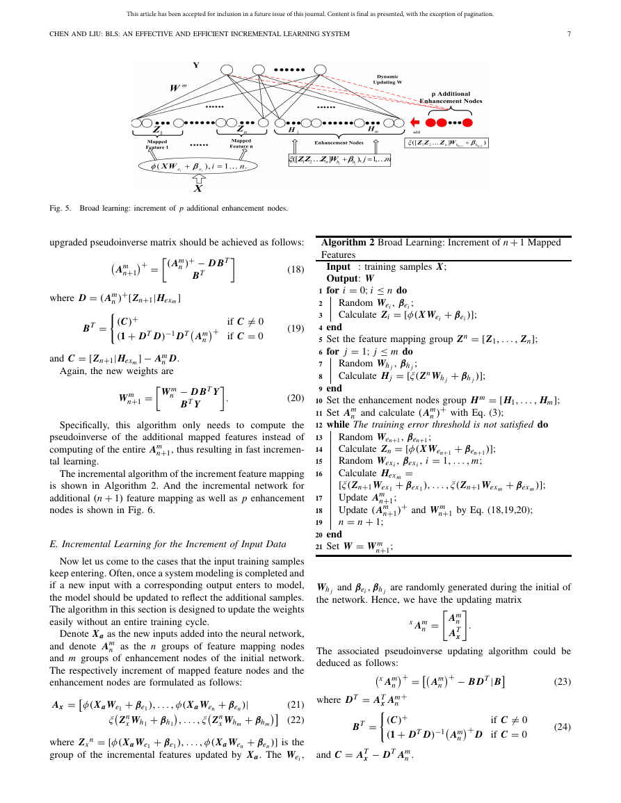
cedure is listed in Algorithm 1, meanwhile, the structure is
illustrated in Fig. 5. Notice that all the peseudoinverse of the
involved matrix are calculated by the regularization approach
in (3). Specifically, this algorithm only needs to compute the
pseudoinverse of the additional enhancement nodes instead of
computations of the entire ( Am+1) and thus results in fast
incremental learning.
The corresponding enhancement nodes are randomly gener-
ated as follows:
+βex1
=[ξ(Zn+1Wex1
|Zn+1|Hexm
+βexm
)] (17)
Hex m
=
n+1
where Wexi and βexi are randomly generated. Denote Am
[ Am
], which is the upgrade of new mapped fea-
tures and the corresponding enhancement nodes. The relatively
), . . . , ξ(Zn+1Wexm
n
�
This article has been accepted for inclusion in a future issue of this journal. Content is final as presented, with the exception of pagination.
CHEN AND LIU: BLS: AN EFFECTIVE AND EFFICIENT INCREMENTAL LEARNING SYSTEM
7
Fig. 5. Broad learning: increment of p additional enhancement nodes.
upgraded pseudoinverse matrix should be achieved as follows:
where D = ( Am
BT =
n
+
Am
n
if C = 0
if C = 0
)+ − D BT
BT
+ =
( Am
n
n+1
Am
)+[Zn+1|Hexm
(C)+
(1 + DT D)−1 DT
]
and C = [Zn+1|Hexm
] − Am
n D.
Again, the new weights are
=
W m
n
n+1
W m
.
− D BT Y
BT Y
(18)
(19)
(20)
Specifically,
this algorithm only needs to compute the
pseudoinverse of the additional mapped features instead of
n+1, thus resulting in fast incremen-
computing of the entire Am
tal learning.
The incremental algorithm of the increment feature mapping
is shown in Algorithm 2. And the incremental network for
additional (n + 1) feature mapping as well as p enhancement
nodes is shown in Fig. 6.
E. Incremental Learning for the Increment of Input Data
Now let us come to the cases that the input training samples
keep entering. Often, once a system modeling is completed and
if a new input with a corresponding output enters to model,
the model should be updated to reflect the additional samples.
The algorithm in this section is designed to update the weights
easily without an entire training cycle.
Ax =
Denote Xa as the new inputs added into the neural network,
and denote Am
n as the n groups of feature mapping nodes
and m groups of enhancement nodes of the initial network.
The respectively increment of mapped feature nodes and the
enhancement nodes are formulated as follows:
)|
+ βhm
+ βen
(21)
(22)
)] is the
where Zx
group of the incremental features updated by Xa. The Wei ,
), . . . , φ(XaWen
+ βh1
+ βe1
+ βe1
Zn
x Wh1
n = [φ(XaWe1
+ βen
Zn
x Whm
φ(XaWe1
), . . . , φ(XaWen
, . . . , ξ
ξ
7
)];
+ βei
: training samples X;
Algorithm 2 Broad Learning: Increment of n + 1 Mapped
Features
Input
Output: W
1 for i = 0; i ≤ n do
Random Wei , βei ;
Calculate Zi = [φ(X Wei
2
3
4 end
5 Set the feature mapping group Zn = [Z1, . . . , Zn];
6 for j = 1; j ≤ m do
Random Wh j , βh j ;
Calculate Hj = [ξ(ZnWh j
8
9 end
10 Set the enhancement nodes group Hm = [H1, . . . , Hm];
11 Set Am
12 while The training error threshold is not satisfied do
13
14
15
16
Random Wen+1, βen+1;
Calculate Zn = [φ(X Wen+1
+ βen+1
Random Wex i , βex i , i = 1, . . . , m;
Calculate Hex m
[ξ(Zn+1Wex1
n+1;
Update Am
n+1
Update ( Am
n = n + 1;
19
20 end
21 Set W = W m
+ βex m
n+1 by Eq. (18,19,20);
=
+ βex 1
)+
), . . . , ξ(Zn+1Wexm
n and calculate ( Am
n
with Eq. (3);
+ βh j
and W m
)];
)];
)];
)+
17
18
n+1;
Wh j and βei
the network. Hence, we have the updating matrix
, βh j are randomly generated during the initial of
.
Am
n
AT
x
=
x Am
n
Am
n
+ =
+ − B DT|B
The associated pseudoinverse updating algorithm could be
deduced as follows:
x Am
n
where DT = AT
+
x Am
n
(C)+
BT =
(1 + DT D)−1
and C = AT
x − DT Am
n .
if C = 0
D if C = 0
+
(24)
Am
n
(23)
�
This article has been accepted for inclusion in a future issue of this journal. Content is final as presented, with the exception of pagination.
8
IEEE TRANSACTIONS ON NEURAL NETWORKS AND LEARNING SYSTEMS
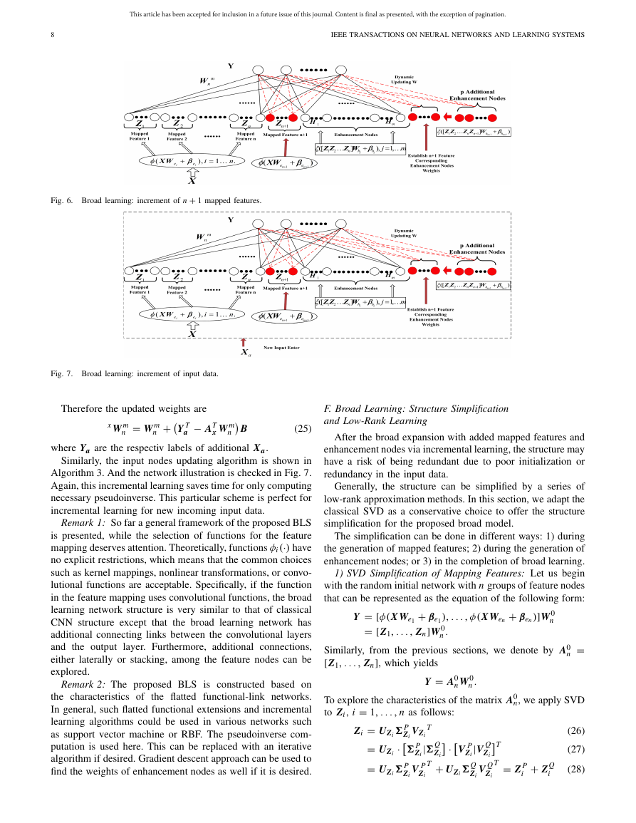
Fig. 6. Broad learning: increment of n + 1 mapped features.
Fig. 7. Broad learning: increment of input data.
Therefore the updated weights are
x W m
n
= W m
n
+
a − AT
Y T
x W m
n
B
(25)
where Ya are the respectiv labels of additional Xa.
Similarly, the input nodes updating algorithm is shown in
Algorithm 3. And the network illustration is checked in Fig. 7.
Again, this incremental learning saves time for only computing
necessary pseudoinverse. This particular scheme is perfect for
incremental learning for new incoming input data.
Remark 1: So far a general framework of the proposed BLS
is presented, while the selection of functions for the feature
mapping deserves attention. Theoretically, functions φi (·) have
no explicit restrictions, which means that the common choices
such as kernel mappings, nonlinear transformations, or convo-
lutional functions are acceptable. Specifically, if the function
in the feature mapping uses convolutional functions, the broad
learning network structure is very similar to that of classical
CNN structure except that the broad learning network has
additional connecting links between the convolutional layers
and the output
layer. Furthermore, additional connections,
either laterally or stacking, among the feature nodes can be
explored.
Remark 2: The proposed BLS is constructed based on
the characteristics of the flatted functional-link networks.
In general, such flatted functional extensions and incremental
learning algorithms could be used in various networks such
as support vector machine or RBF. The pseudoinverse com-
putation is used here. This can be replaced with an iterative
algorithm if desired. Gradient descent approach can be used to
find the weights of enhancement nodes as well if it is desired.
F. Broad Learning: Structure Simplification
and Low-Rank Learning
After the broad expansion with added mapped features and
enhancement nodes via incremental learning, the structure may
have a risk of being redundant due to poor initialization or
redundancy in the input data.
Generally, the structure can be simplified by a series of
low-rank approximation methods. In this section, we adapt the
classical SVD as a conservative choice to offer the structure
simplification for the proposed broad model.
The simplification can be done in different ways: 1) during
the generation of mapped features; 2) during the generation of
enhancement nodes; or 3) in the completion of broad learning.
1) SVD Simplification of Mapping Features: Let us begin
with the random initial network with n groups of feature nodes
that can be represented as the equation of the following form:
+ βe1
Y = [φ(X We1
= [Z1, . . . , Zn]W 0
Similarly, from the previous sections, we denote by A0
[Z1, . . . , Zn], which yields
n
), . . . , φ(X Wen
.
+ βen
)]W 0
n
n
=
.
nW 0
n
Y = A0
To explore the characteristics of the matrix A0
to Zi , i = 1, . . . , n as follows:
·
|� Q
Zi
T + UZi
Zi = UZi
= UZi
= UZi
·
Zi VZi
� P
Zi
� P
Zi V P
Zi
T
T = Z P
|V Q
Zi
V Q
Zi
V P
Zi
� Q
Zi
� P
T
i
n, we apply SVD
(26)
(27)
(28)
+ Z Q
i
�




 2023年江西萍乡中考道德与法治真题及答案.doc
 2012年重庆南川中考生物真题及答案.doc
 2013年江西师范大学地理学综合及文艺理论基础考研真题.doc
 2020年四川甘孜小升初语文真题及答案I卷.doc
 2020年注册岩土工程师专业基础考试真题及答案.doc
 2023-2024学年福建省厦门市九年级上学期数学月考试题及答案.doc
 2021-2022学年辽宁省沈阳市大东区九年级上学期语文期末试题及答案.doc
 2022-2023学年北京东城区初三第一学期物理期末试卷及答案.doc
 2018上半年江西教师资格初中地理学科知识与教学能力真题及答案.doc
 2012年河北国家公务员申论考试真题及答案-省级.doc
 2020-2021学年江苏省扬州市江都区邵樊片九年级上学期数学第一次质量检测试题及答案.doc
 2022下半年黑龙江教师资格证中学综合素质真题及答案.doc