Feature
Reinforcement
Learning and Adaptive
Dynamic Programming
for Feedback Control
Frank L. Lewis
and Draguna Vrabie
Abstract
Living organisms learn by
acting on their environ-
ment, observing the re-
sulting reward stimulus,
and adjusting their actions
accordingly to improve
the reward. This action-
based or Reinforcement
Learning can capture no-
tions of optimal behavior
occurring in natural sys-
tems. We describe math-
ematical formulations for
Reinforcement Learning
and a practical implemen-
tation method known as
Adaptive Dynamic Pro-
gramming. These give us
insight into the design of
controllers for man-made
engineered systems that
both learn and exhibit op-
timal behavior.
Digital Object Identifier 10.1109/MCAS.2009.933854
32
IEEE CIRCUITS AND SYSTEMS MAGAZINE
1531-636X/09/$26.00©2009 IEEE
THIRD QUARTER 2009
I
S
E
R
U
T
C
P
X
D
N
A
R
B
©
�
Reinforcement Learning and
Optimality in Nature
Every living organism interacts with its environment
and uses those interactions to improve its own ac-
tions in order to survive and increase. Charles
Darwin showed that species modify their actions based
on interactions with the environment over long time
scales, leading to natural selection and survival of the
fittest. Adam Smith showed that modification of the ac-
tions of corporate entities based on interactions on the
scale of a global economy is responsible for the relative
balance and wealth of nations. Ivan Pavlov used simple
reinforcement and punishment stimuli to modify the be-
havior patterns of dogs by inducing conditional reflexes.
We call modification of actions based on interac-
tions with the environment reinforcement learning
(RL) [Mendel 1970]. There are many types of learning
including supervised learning, unsupervised learning,
etc. Reinforcement learning refers to an actor or agent
that interacts with its environment and modifi es its
actions, or control policies, based on stimuli received
in response to its actions. This is based on evaluative
information from the environment and could be called
action-based learning. RL implies a cause and effect re-
lationship between actions and reward or punishment.
It implies goal directed behavior at least insofar as the
agent has an understanding of reward versus lack of
reward or punishment.
The RL algorithms are constructed on the idea that
successful control decisions should be remembered, by
means of a reinforcement signal, such that they become
more likely to be used a second time. Although the idea
originates from experimental animal learning, where it
has been observed that the dopamine neurotransmitter
acts as a reinforcement informational signal which fa-
vors learning at the level of the neuron (see e.g., [Shultz
et al. 1997, 2004], [Doya 2001]), RL is strongly connected
from a theoretical point of view with direct and indirect
adaptive optimal control methods.
One class of reinforcement learning methods is based
on the Actor-Critic structure [Barto, Sutton, Anderson
1983], where an actor component applies an action or
control policy to the environment, and a critic compo-
nent assesses the value of that action. Based on this as-
sessment of the value, various schemes may then be used
to modify or improve the action in the sense that the new
policy yields a value that is improved over the previous
value. The actor-critic structure implies two steps: policy
evaluation by the critic followed by policy improvement.
The policy evaluation step is performed by observing
from the environment the results of current actions.
The limits within which organisms can survive are
often quite narrow and the resources available to most
species are meager. Therefore, most organisms act in
an optimal fashion to conserve resources yet achieve
their goals. Optimal actions may be based on minimum
fuel, minimum energy, minimum risk, maximum reward,
and so on. Therefore, it is of interest to study reinforce-
ment learning systems having an actor-critic structure
wherein the critic assesses the value of current policies
based on some sort of optimality criteria [Werbos 1974,
1989, 1991, 1992], [Bertsekas 1996], [Sutton and Barto
1998], [Cao 2009]. In the optimal RL algorithms case
the learning process is moved to a higher level having
no longer as object of interest the details of a system’s
dynamics, but a performance index which quantifies
how close to optimality does the closed loop control
system operate. In such a scheme, reinforcement learn-
ing is a means of learning optimal behaviors by observ-
ing the response from the environment to nonoptimal
control policies.
Feedback Control Theory is the study of means of
developing control systems for human engineered sys-
tems to endow them with guaranteed performance and
safety. Included are control systems for aircraft, ships,
race cars, robot systems, industrial processes, building
temperature and climate regulation systems, and many
more. It is often of interest to mimic nature and design
control systems that are optimal in some sense of ef-
fectively achieving required performance without using
undue amounts of resources.
The purpose of this article is to show the usefulness
of reinforcement learning techniques, specifically a fam-
ily of techniques known as Approximate or Adaptive
Dynamic Programming (ADP) (also known as Neurody-
namic Programming), for the feedback control of human
engineered systems. Reinforcement learning techniques
have been developed by the Computational Intelligence
Community. Therefore, this requires bringing together
ideas from two communities-Control Systems Engineer-
ing and Computational Intelligence. Since reinforcement
learning involves modifying the control policy based on
responses from the environment, one has the initial feel-
ing that it should be closely related to adaptive control,
a family of successful control techniques held in high
regard in Control Systems Community.
The intention here is to present the main ideas and al-
gorithms of reinforcement learning Approximate Dynam-
ic Programming, not give a literature survey or historical
development. Very good surveys are given in [Si et al.
2004], the recent IEEE Transactions on SMC Part B spe-
cial issue [Lewis, Lendaris, Liu 2008], [Balakrishnan et al.
Frank L. Lewis and Draguna Vrabie are with the Automation & Robotics Research Institute, The University of Texas at Arlington.
THIRD QUARTER 2009
IEEE CIRCUITS AND SYSTEMS MAGAZINE
33
�
intelligence notions including policy iteration and value
iteration. Then, we illustrate using the linear quadratic
regulator (LQR) case to show that these notions are in
fact familiar in the feedback control theory setting. After
that, we proceed to develop online reinforcement learn-
ing schemes for DT dynamical systems. These latter
ideas have not been fully exploited in the control sys-
tems community.
Optimal Control for
Discrete-Time Systems
There are standard methods for sampling or discretizing
nonlinear continuous-time state space ODEs to obtain
sampled data forms that are convenient for computer-
based control [Lewis and Syrmos 1995]. The resulting
systems unfold in discrete time and are generally of the
state-space form xk11 5 F1xk, uk
2 with k the discrete time
index. These systems satisfy the 1-step Markov property
since their state at time k 1 1only depends on the state
and inputs at the previous time k.
For ease of analysis one often considers a class of
discrete-time systems described by nonlinear dynamics
in the affine state space difference equation form
xk11 5 f1xk
2 1 g1xk
2uk
with state xk [ Rn and control input uk [ Rm. The analy-
sis of such forms is convenient and can be generalized
to the general sampled data form xk11 5 F1xk, uk
space to control space h1.2:Rn S Rm. That is, for every
A control policy is defined as a function from state
2.
state xk, the policy defines a control action
uk 5 h1xk
2.
2008], and the recent article [Wang, Zhang, Liu 2009].
A biography is included here for further reference by
the reader.
Dynamical Systems and
Optimal Feedback Control
In the study and design of feedback control systems it
is required to provide design algorithms and analysis
techniques that yield guaranteed provable performance
and safety margins. Feedback controllers without per-
formance, stability, and robustness guarantees will not
be accepted by industry. A standard means for providing
such guarantees is to use the framework and tools pro-
vided by mathematics. Thus, to be precise, we should
like to capture the ideas about reinforcement learning
in some sort of mathematical formulation. One such for-
mulation is the framework of Markov decision processes
(MDP). MDP have been extensively used to study and
embody reinforcement learning systems. In MDP, the
state spaces and action spaces are generally discrete
(i.e. state and action take on only certain allowed dis-
crete values). However, human engineered systems de-
velop and move through time and generally have states
and actions that reside in continuous spaces. A broad
class of engineered systems can be effectively described
by ordinary differential equations, since these describe
the development of a system through time based on its
current status as well as any inputs received, such as
commands, disturbances, and so on.
Dynamical Systems
Physical analysis of dynamical systems using Lagrang-
ian mechanics, Hamiltonian mechanics, etc. produces
system descriptions in terms of nonlinear ordinary dif-
ferential equations. Particularly prevalent are nonlinear
#
ODEs in the state-space form x
5 f1x, u2, with the state
x1t2 [ Rn and control input u1t2 [ Rm residing in contin-
uous spaces. Many systems in aerospace, the automo-
tive industry, process industry, robotics, and elsewhere
are conveniently put into this form. In addition to being
continuous-state space and continuous-input space sys-
tems, in contrast to MDP which have discrete states and
actions, these dynamics are also continuous-time (CT)
systems. For nonlinear systems, the PI algorithm was
first developed by Leake and Liu (1967). Three decades
later it was introduced in (Beard, Saridis, and Wen,
1997) as a feasible adaptive solution to the CT optimal
control problem.
The bulk of research in ADP has been conducted for
systems that operate in discrete-time (DT). Therefore, we
cover DT systems first, then continuous-time systems.
Here, we first consider nonlinear DT systems and out-
line DT optimal control, developing some computational
(1)
(2)
Such mappings are also known as feedback controllers.
An example policy is a linear state-variable feedback
2 5 2 Kxk. Another example policy is a transfer
uk 5 h1xk
function dynamical controller design. In the feedback
controls community, the feedback control policy can be
designed using many methods including optimal control
via solution of the Riccati equation, adaptive control,
H-infinity control, classical frequency domain control, etc.
In reinforcement learning, the control policy is learned
in real time based on stimuli received from the environ-
ment. Clearly, this learning sort of controller design is re-
lated to notions of adaptive control, as we shall see.
System or Environment? In reinforcement learning,
the actor is the agent that generates the control policy.
That is, the actor is mathematically described by the
policy (2), which has the state x1t2 as input and the
control u1t2as output. Everything outside the actor is
considered to be the environment. Thus, the system (1)
is considered as part of the environment, as are all
disturbances and extraneous effects. In fact, in standard
34
IEEE CIRCUITS AND SYSTEMS MAGAZINE
THIRD QUARTER 2009
�
applications of reinforcement learning, the system dy-
namics is not even considered, and as part of the en-
vironment, no explicit model of the dynamics, such as
(1), is even used. Reinforcement learning has enjoyed
rather remarkable successes for complex systems with
unknown dynamics, including the backgammon player
of Tesauro, and the design of controllers that can back
up truck tractor/trailer rigs with multiple concatenated
trailers. However, not specifically considering the dy-
namics also makes it impossible to provide explicit
proofs of stability and performance such as are required
for acceptance by the Control Systems Community.
Goal Directed Optimal Performance
The notion of goal-directed optimal behavior is captured
by defining a performance measure or cost function
Vh
1xk
2 5 a
`
gi2kr1xi, ui
2
(3)
2 a pre-
with 0 , g # 1 a discount factor and uk 5 h1xk
i5k
scribed feedback control policy. This is known as the
cost-to-go and is a sum of discounted future costs from
the current time k into the infinite horizon future. The
discount factor reflects the fact that we are less con-
cerned about costs acquired further into the future.
2 is known as the utility, and is a mea-
Function r1xk, uk
sure of the one-step cost of control. This can be selected
based on minimum-fuel considerations, minimum ener-
gy, minimum risk, etc. For instance, a standard form is
TRuk
the quadratic energy function r1xk, uk
2 1 uk
or the more general form
2 5 Q1xk
r1xk, uk
2 5 xk
TQxk 1 uk
TRuk,
The objective of optimal control theory is to select
the policy that minimizes the cost to obtain
V * 1xk
2 5 min
h1#2 a a
`
i5k
gi2kr1xi, h1xi
22b
(5)
which is known as the optimal cost, or optimal value.
Then, the optimal control policy is given by
h*1xk
2 5 arg min
h1#2
`
a a
i5k
gi2kr1xi, h1xi
22b
(6)
A short-sighted or myopic planner would only be
concerned about minimizing the one-step cost or util-
2. However, the problem is to minimize not
ity r1xk, uk
simply the one-step cost, but the sum of all discounted
costs, or the cost-to-go. This problem is generally very
difficult or even impossible to solve exactly for general
nonlinear systems.
Note that in computational intelligence, (3) is often in-
terpreted as a reward, and the objective is to maximize it.
Various methods have been developed to simplify
the solution of this optimization problem. Some of these
are known within the Control Systems Community and
some within the Computational Intelligence Community.
We shall discuss:
■
■
■
Bellman’s optimality principle and dynamic pro-
gramming
Policy iteration and value iteration
Various forms of reinforcement learning based on
temporal differences and ADP.
Bellman’s Optimality Principle and
Dynamic Programming
By writing (3) as
(4)
which we use at times for illustration. We require
Q1x2, R to be positive definite so that the cost function
1xk
2 5 r1xk, uk
Vh
is well defined.
2 1 g a
`
gi21k112
r1xi, ui
2,
(7)
i5k11
We assume the system is stabilizable on some set
V [ Rn, that is there exists a control policy uk 5 h1xk
such that the closed-loop system xk115 f1xk
2h1xk
is asymptotically stable on V. A control policy uk 5 h1xk
2 its
1xk
For any admissible policy uk 5 h1xk
is said to be admissible if it is stabilizing and yields a
finite cost Vh
2, we call Vh
2 1 g1xk
1xk
2
2
2
2.
cost or value. Policies with smaller values are deemed to
be better than others. It is important to note that, given
any admissible policy, its value may be determined by
evaluating the infinite sum (3). This may be done by ex-
plicit computation in some cases, or by simulation using
a digital computer, or by actual evaluation in real-time by
observing the trajectories of the closed-loop system.
The means by which the value or cost of a control pol-
icy is determined is one of the key differences between
feedback control theory and reinforcement learning.
one sees that a difference equation equivalent to is
given by
1xk
2 5 r1xk, h1xk
22 1 gVh
1xk11
2, Vh
102 5 0.
Vh
(8)
That is, instead of evaluating the infinite sum (3), one
can solve the difference equation to obtain the value of
using a current policy uk 5 h1xk
2.
This is a nonlinear Lyapunov equation known as
the Bellman equation. Evaluating the value of a current
policy using the Bellman equation is the first key con-
cept in developing reinforcement learning techniques,
as we shall see. Then, we shall show how to solve the
Bellman equation on-line in real-time using observed
data from the system trajectories.
The DT Hamiltonian can be defi ned as
H1xk, h1xK
2, DVk
2 5 r1xk, h1xk
22 1gVh
1xk11
2 2Vh
1xk
2, (9)
THIRD QUARTER 2009
IEEE CIRCUITS AND SYSTEMS MAGAZINE
35
�
1xk11
2 2 Vh
1xk
2 is the forward difference
where DVk 5 gVh
operator. The Hamiltonian function captures the energy
content along the trajectories of a system as reflected in
the desired optimal performance. The Bellman equation
requires that the Hamiltonian be equal to zero for the
value associated with a prescribed policy.
The optimal value can be written using the Bellman
equation as
*1xk
2 5 min
h1#2
1r1xk, h1xk
22 1 gVh
1xk11
22.
(10)
V
This optimization problem is still difficult to solve.
Bellman’s principle [Bellman 1957] is a cornerstone
of optimal control, and states that “An optimal policy
has the property that no matter what the previous deci-
sions (i.e. controls) have been, the remaining decisions
must constitute an optimal policy with regard to the
state resulting from those previous decisions”. In terms
of equations, this means that
V *1xk
2 5 min
h1#2
1r1xk, h1xk
22 1 gV *1xk11
22.
(11)
This is known as the Bellman optimality equation, or the
discrete-time Hamilton-Jacobi-Bellman (HJB) equation.
One then has the optimal policy as
1r1xk, h1xk
22 1 gV *1xk11
22.
(12)
h*1xk
2 5 arg min
h1.2
Determining optimal controllers using these equations is
considerably easier than by using (10), since they contain
the optimal value inside the minimization argument.
Since one must know the optimal policy at time k 1 1
to (11) use to determine the optimal policy at time k,
Bellman’s Principle yields a backwards-in-time procedure
for solving the optimal control problem. It is the basis for
Dynamic Programming algorithms in extensive use in con-
trol system theory, Operations Research, and elsewhere.
These are by nature off-line planning methods. An example
of such a procedure in feedback controls design is Riccati
equation design for the LQR problem, which involves off-
line solution of the Riccati equation given known system
dynamics (see below). DP methods generally require the
full knowledge of the system dynamical equations. That is
f1x2, g1x2 must be known.
Policy Iteration, Value Iteration,
and Fixed Point Equations
In contrast to dynamic programming off-line designs, we
seek reinforcement learning schemes for on-line learning in
real time, ultimately without knowing the system dynamics
f1x2, g1x2. Therefore, we next show how to exploit the no-
tion that the Bellman equation and the Bellman optimality
equation (11) are fixed point equations to develop forward-
in-time methods for solving the optimal control problem.
We are now in a position to use these constructions as
a foundation for reinforcement learning optimal control.
2 5 arg min
h1#2
Consider any given admissible policy uk 5 h1xk
ue Vh
mine a new policy from this value using the operation
2 with val-
1xk
2. Motivated, though not justified, by (12) deter-
hr1xk
1r1xk, h1xk
is shown that the new policy hr1xk
it has value Vhr1xk
1xk
22 1 gVh
2 is improved in that
2 less than or equal to the old value
2. This is known as the one step improvement prop-
Vh
erty of rollout algorithms. That is, the step (13) has giv-
en an improved policy.
This procedure is justified in Bertsekas [1996], where it
1xk11
22.
(13)
This suggests the following iterative method for de-
termining the optimal control, which is known as Policy
Iteration [Leake and Liu 1967], [Sutton and Barto 1998],
[Bertsekas 1996]. See Figure 3.
Policy Iteration (PI) Algorithm
2
1xk
Initialize. Select any admissible (i.e. stabilizing) con-
trol policy h0
Policy Evaluation Step. Determine the value of the
current policy using the Bellman Equation
1xk
2 5 r1xk, hj
1xk
22 1 gVj11
1xk11
Vj11
(14)
Policy Improvement Step. Determine an improved
policy using
22. (15)
1r1xk, h1xk
22 1 gVj11
1xk11
1xk
2 5 arg min
h1#2
hj11
2.
g
2
(16)
If the utility has the special form and the dynamics are
(1), then the policy improvement step looks like
1xk
2 5 2
R21gT1xk
2 =Vj11
1xk11
2,
hj11
where =V1x2 5 'V1x2 /'x is the gradient of the value func-
tion, interpreted here as a column vector.
Note that the initial policy in PI must be admissible,
which requires that it be stabilizing. It has been shown
by [Leake and Liu 1967], [Howard 1960] and others that
this algorithm converges under certain conditions to
the optimal value and control policy, that is, to the solu-
tion of (11), (12).
The evaluation of the value of the current policy us-
ing the Bellman Equation (14) amounts to determining
the value of using the policy hj
rent states xk. This is called a full backup in [Sutton and
Barto 1998] and can involve significant computation.
2 starting in all cur-
1xk
uk 5 h1xk
lowing contraction map
In fact, it can be shown that the Bellman equation is a
fixed point equation. That is, given an admissible policy
2, has a unique fixed point Vh
V i111xk
2, and the fol-
1xk
22 1 gV i1xk11
2 5 r1xk, h1xk
2
can be iterated starting with any value V 01xk
2, and there
1xk
2 S Vh
2. Therefore one can re-
results in the limit V i1xk
place the policy iteration step (14) by
36
IEEE CIRCUITS AND SYSTEMS MAGAZINE
THIRD QUARTER 2009
�
1xk
V i111xk
22 1 gV i1xk11
2, for i 5 1, 2, … , (17)
2 5 r1xk, hj
1 #2 until convergence. Then, V i1x2 S Vj11
2 5 Vj
i S `. One generally selects at step j V 01xk11
where the iteration in i is carried out with the same
policy hj
1x2 as
1xk11
2.
This can be called Iterative Policy Iteration [Sutton and
Barto 1998]. It is noted that each step in (17) is far sim-
pler to implement that a single step of (14), as we see
below when we consider the LQR case.
This suggests further the idea of iterating (17) for only
K steps, for a fixed finite integer K. That is, only K steps are
taken towards evaluating the value of the current policy.
This is known as Generalized Policy Iteration in [Sutton and
Barto 1998]. In GPI, at each policy update step, only a par-
tial backup is done of the values. An extreme case is to take
K 5 1, which gives the next algorithm, known as Value Itera-
tion. There, only a 1-step backup of values is performed.
2, not neces-
Value Iteration (VI) Algorithm
1xk
Initialize. Select any control policy h0
sarily admissible or stabilizing.
Value Update Step. Update the value using
2.
2 5 r1xk, hj
22 1 gVj
1xk11
1xk
1xk
Vj11
(18)
Policy Improvement Step. Determine an improved
policy using
22. (19)
1r1xk, h1xk
22 1 gVj11
1xk11
1xk
2 5 arg min
h1#2
hj11
It is important to note that now, the old value is used on the
right-hand side of (14), in contrast to the PI step (14). It has
been shown that VI converges under certain situations.
Note that VI does not require an initial stabilizing policy.
In fact, on further thought, it is seen that Value Iteration
is based on the fact that the Bellman Optimality Equation
(11) is also a fixed point equation. The interleaved steps
of value update and policy improvement are the means of
iterating the contraction map associated to (11).
It is important to note that PI requires at each step
the solution of (14), which is a nonlinear Lyapunov equa-
tion. This solution is difficult for general nonlinear sys-
tems. On the other hand, VI relies on the solution of (18),
which is simply a recursion equation.
Generally, fixed point equations can be used, with
suitable formulation, as a basis for on-line reinforcement
learning algorithms that learn by observing data accrued
along system trajectories. We shall shortly develop re-
inforcement learning schemes based on these notions.
First, to pin down ideas, let us consider the LQR case.
The DT Linear Quadratic
Regulator (LQR) Case
The main purpose of this section is to show that the rein-
forcement learning notions of Policy Iteration and Value
Iteration are in fact in line with familiar ideas in feedback
control systems. A second purpose is to give explicit for-
mulae for the above constructions for an important class
of problems that illustrates further their meaning.
A large class of important discrete-time (DT) sys-
tems can be described in the linear time invariant state-
space form
xk11 5 Axk 1 Buk
(20)
with state xk [ Rn and control input uk [ Rm. The control
policies of interest are then state variable feedbacks of
the form
uk 5 h1xk
2 5 2 Kxk
(21)
with the control policy a constant feedback gain matrix
K to be determined.
Given a prescribed policy, the cost function is the
sum of quadratic functions
1xk
Vh
2 5 a
`
i5k
`
5 a
i5k
2
TQxi 1 ui
1xi
T1Q 1K TRK2xi ; VK
TRui
xi
1xk
2,
(22)
which has utility r1xk, uk
2 5 xk
TRuk with weight-
ing matrices Q 5 QT $ 0, R 5 RT . 0. It is assumed that
(A, B) is stabilizable, i.e., there exists a feedback gain
matrix K such that the closed-loop system
TQxk 1 uk
xk11 5 1A 2 BK2xk ; Acxk
is asymptotically stable. It is also assumed that 1A, "Q2
is detectable, i.e. "Q xk
S 0 implies that xk
S 0.
(23)
Optimal Control Solution for the DT LQR
The objective of this design is to select the state feed-
back gain K, i.e. the control policy, to minimize the
cost-to-go Vh
is called the linear quadratic regulator (LQR) problem
[Lewis and Syrmos 1995].
2 for all current states xk. This
2 5 VK
1xk
1xk
It can be shown that the optimal value for the LQR is
quadratic in the current state so that
V *1xk
2 5 xk
TPxk
(24)
for some matrix P, which is to be determined. Therefore,
the Bellman equation for the LQR is
TPxk 5 xk
xk
TQxk 1 uk
TRuk 1 xk11
T Pxk11.
(25)
In terms of the feedback gain this can be written as
T1Q 1 KTRK 1 1A 2 BK2 TP1A 2 BK22xk. (26)
TPxk 5 xk
xk
Since this must hold for all current states xk one has
1A 2 BK2 T P1A 2 BK2 2 P 1 Q 1 KTRK 5 0.
(27)
THIRD QUARTER 2009
IEEE CIRCUITS AND SYSTEMS MAGAZINE
37
�
Every living organism interacts with its environment and uses those interactions
to improve its own actions in order to survive and increase.
This matrix equation is linear in P and is known as a
Lyapunov equation when K is fixed. Solving this equation
given a prescribed stabilizing gain K yields P 5 PT . 0
TPxk is the cost of using the policy
such that VK
K. That is,
VK
T1Q 1 K TRK2xi 5 xk
xi
TPxk.
(28)
1xk
2 5 xk
1xk
2 5 a
`
i5k
The equations and are easily solved for the LQR. Write
the Bellman equation as
xk
TPxk 5 xk
TQxk 1 uk
TRuk 11Axk 1 Buk
2 TP1Axk 1 Buk
2, (29)
whence the minimization is easily performed by differ-
entiating with respect to uk to obtain
2 5 0
Ruk 1 BTP1Axk 1 Buk
uk 521R 1 BTPB2 21BTPAxk,
or
(30)
(31)
so the optimal feedback gain is
K 5 1R 1 BTPB2 21BTPA.
Substituting this into the Bellman equation (29) and
simplifying yields the DT HJB equation
ATPA 2 P 1 Q 2 ATPB1R 1 BTPB2 21BTPA 5 0. (32)
This equation is quadratic in P and is known as the
Riccati equation.
To solve the DT LQR optimal control problem, one first
solves the Riccati equation for P, then the optimal value is
given by V *1xk
2 5 xk
TPxk and the optimal policy by (31).
On-line learning vs. off-line planning solution
of the LQR. It is important to note the following key
point. In going from the formulation (25) of the Bell-
man equation to the formulation (27), which is the Ly-
apunov equation, one has performed two steps. First,
the system dynamics are substituted for xk11 to yield
(26), next the current state xk is cancelled to obtain
(27). These two steps make it impossible to apply
real-time online reinforcement learning methods to
find the optimal control, which we shall do in the next
section. Because of these two steps, optimal controls
design in the Control Systems Community is almost
universally an off-line procedure involving solutions
of Riccati equations, where full knowledge of the sys-
tem dynamics 1A, B2 is required.
Policy Iteration and Value Iteration
for the DT LQR
We will now see that Policy Iteration and Value Iteration
are actually well known in the Control Systems Commu-
nity, though there they are called something else, name-
ly Hewer’s method for solving the DT Riccati equation
[Hewer 1971].
For the LQR, Bellman’s equation (8) is written as (25)
and hence is equivalent to the Lyapunov equation (32).
Therefore, in the Policy Iteration Algorithm, the policy
evaluation step for LQR is
1A 2 BKj
2 TPj11
1A 2 BKj
2 2 Pj11 1 Q 1 Kj
TRKj 5 0. (33)
and the policy update is
Kj11 5 1R 1 BT Pj11B2 21 BT Pj11A.
(34)
However, iteration of these two equations is exactly
Hewer’s algorithm [Hewer 1971] to solve the Riccati
equation (32). Hewer proved that it converges under the
stabilizability and detectability assumptions.
In the Value Iteration Algorithm, the policy evalua-
tion step for LQR is
Pj11 5 1A 2 BKj
2 TPj
1A 2 BKj
2 1 Q 1 Kj
TRKj.
(35)
and the policy update (29) is (34). However, iteration
of these two equations has been studied by Lancaster
and Rodman [1995], who showed that it converges to the
Riccati equation solution under the stated assumptions.
Note that Policy Iteration involves full solution of a
Lyapunov equation (33) at each step and requires a sta-
bilizing gain Kj at each step. This is called a full backup
in reinforcement learning terms. On the other hand, Val-
ue Iteration involves only a Lyapunov recursion (35) at
each step, which is very easy to compute, and does not
require a stabilizing gain. This is called a partial backup
in reinforcement learning.
The recursion (35) can be performed even if Kj is not
stabilizing. If Kj is in fact stabilizing, then iterating the
Lyapunov recursion (35), with a fixed feedback gain Kj,
until convergence provides the solution to the Lyapunov
equation (33).
Reinforcement Learning suggests another algorithm
for solving the Riccati equation, namely Generalized
Policy Iteration. In GPI, one would perform the following
at each step.
38
IEEE CIRCUITS AND SYSTEMS MAGAZINE
THIRD QUARTER 2009
�
The means by which the value or cost of a control policy is determined
is one of the key differences between feedback control theory and
reinforcement learning.
Generalized Policy Algorithm for LQR
Initialize. Select any control policy K0, not necessar-
ily admissible or stabilizing.
Value Update Step. At step j, update the value using
i11 51A 2 BKj
Pj
2TPj
i1A2BKj
2 1 Q 1 Kj
TRKj,
i 50, 1, ..., K 2 1
(36)
for some finite K, setting as initial condition Pj
K.
Set Pj11 5 Pj
Policy Improvement Step. Determine an improved
policy using
0 5 Pj.
Kj11 5 1R 1 BTPj11B2 21BTPj11A.
(37)
This algorithm takes K steps towards solving the
Lyapunov equation at each iteration j. That is, the value
update step in GPI consists of K steps of the recursion
(35) using the same fixed gain. Setting K 5 1 yields Value
Iteration, i.e. (35), whereas setting K 5 ` (i.e. perform
(36) until convergence) yields Policy Iteration, which
solves the Lyapunov equation (33).
Reinforcement Learning, ADP, and
Adaptive Control
The optimal control solution using dynamic program-
ming is a backwards-in-time procedure. Therefore, it can
be used for off-line planning but not online learning. We
have seen that the Bellman equation (8) leads to several
iterative methods for learning the solution of the opti-
mal control equation without solving the HJB equation,
including Policy Iteration and Value Iteration. In this
section we shall see how to formulate these as on-line
real-time reinforcement learning methods for solving the
optimal control problem using data measured along sys-
tem trajectories [Sutton and Barto 1998]. These methods
are broadly called approximate dynamic programming
(ADP) [Werbos 1974, 1989, 1991, 1992] or neurodynamic
programming (NDP) [Bertsekas 1996]. There are two key
ingredients: temporal difference (TD) error and value
function approximation (VFA).
The Bellman equation is a fixed point equation which
can be viewed as a consistency equation that the value
must satisfy if it is consistent with the current control
policy. Generally, fixed point equations can be used,
with suitable formulation, as a basis for reinforcement
learning algorithms. Let us now develop on-line rein-
forcement learning schemes based on these notions.
ADP-Temporal Difference (TD) and
Value Function Approximation (VFA)
Approximate Dynamic Programming (ADP), or Neuro-
dynamic Programming (NDP), is a practical method for
determining the optimal control solution online forward
in time by using measured system data along the sys-
tem trajectories. It is based on providing methods for
solving the dynamic programming problem forward in
time in real-time and for approximating the value func-
tion. References are the work of Sutton and Barto [1998],
Werbos [1974, 1989, 1991, 1992], and Bertsekas [1996].
Temporal Difference (TD) Error. To turn these con-
cepts into forward-in-time online solution methods,
based on the Bellman equation define a time-varying
residual equation error as
ek 5 r1xk, h1xk
22 1 gVh
1xk11
2 2 Vh
1xk
2.
(38)
One notes that the right-hand side of this is the DT Ham-
iltonian function. Function ek is known as the tempo-
ral difference error. If the Bellman equation holds, the
TD error is zero. Therefore, for a fixed control policy
u 5 h1x2one may solve the equation ek 5 0 at each time
1 #2 that is the least-squares
k for the value function Vh
solution to the TD equation
0 5 r1xk, h1xk
22 1 gVh
1xk11
2 2 Vh
1xk
2.
(39)
This yields the best approximation to the value correspond-
ing to using the current policy, i.e. to the summation (3).
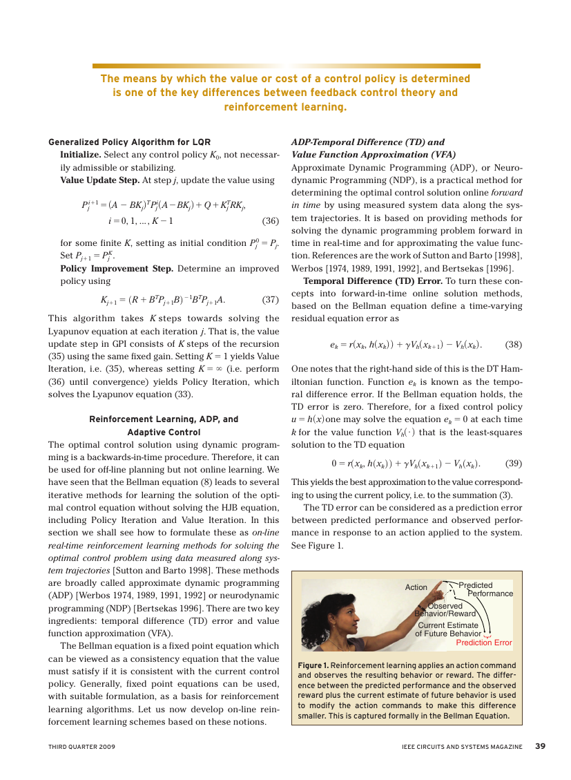
The TD error can be considered as a prediction error
between predicted performance and observed perfor-
mance in response to an action applied to the system.
See Figure 1.
Action
Predicted
Performance
Observed
Behavior/Reward
Current Estimate
of Future Behavior
Prediction Error
Figure 1. Reinforcement learning applies an action command
and observes the resulting behavior or reward. The differ-
ence between the predicted performance and the observed
reward plus the current estimate of future behavior is used
to modify the action commands to make this difference
smaller. This is captured formally in the Bellman Equation.
THIRD QUARTER 2009
IEEE CIRCUITS AND SYSTEMS MAGAZINE
39
�


 2023年江西萍乡中考道德与法治真题及答案.doc
 2012年重庆南川中考生物真题及答案.doc
 2013年江西师范大学地理学综合及文艺理论基础考研真题.doc
 2020年四川甘孜小升初语文真题及答案I卷.doc
 2020年注册岩土工程师专业基础考试真题及答案.doc
 2023-2024学年福建省厦门市九年级上学期数学月考试题及答案.doc
 2021-2022学年辽宁省沈阳市大东区九年级上学期语文期末试题及答案.doc
 2022-2023学年北京东城区初三第一学期物理期末试卷及答案.doc
 2018上半年江西教师资格初中地理学科知识与教学能力真题及答案.doc
 2012年河北国家公务员申论考试真题及答案-省级.doc
 2020-2021学年江苏省扬州市江都区邵樊片九年级上学期数学第一次质量检测试题及答案.doc
 2022下半年黑龙江教师资格证中学综合素质真题及答案.doc