6
1
0
2
r
a
M
9
2
]
G
L
.
s
c
[
4
v
9
3
9
6
0
.
1
1
5
1
:
v
i
X
r
a
Published as a conference paper at ICLR 2016
SESSION-BASED RECOMMENDATIONS WITH
RECURRENT NEURAL NETWORKS
Bal´azs Hidasi ∗
Gravity R&D Inc.
Budapest, Hungary
balazs.hidasi@gravityrd.com
Alexandros Karatzoglou
Telefonica Research
Barcelona, Spain
alexk@tid.es
Linas Baltrunas †
Netflix
Los Gatos, CA, USA
lbaltrunas@netflix.com
Domonkos Tikk
Gravity R&D Inc.
Budapest, Hungary
domonkos.tikk@gravityrd.com
ABSTRACT
We apply recurrent neural networks (RNN) on a new domain, namely recom-
mender systems. Real-life recommender systems often face the problem of having
to base recommendations only on short session-based data (e.g. a small sportsware
website) instead of long user histories (as in the case of Netflix). In this situation
the frequently praised matrix factorization approaches are not accurate. This prob-
lem is usually overcome in practice by resorting to item-to-item recommendations,
i.e. recommending similar items. We argue that by modeling the whole session,
more accurate recommendations can be provided. We therefore propose an RNN-
based approach for session-based recommendations. Our approach also considers
practical aspects of the task and introduces several modifications to classic RNNs
such as a ranking loss function that make it more viable for this specific problem.
Experimental results on two data-sets show marked improvements over widely
used approaches.
1
INTRODUCTION
Session-based recommendation is a relatively unappreciated problem in the machine learning and
recommender systems community. Many e-commerce recommender systems (particularly those
of small retailers) and most of news and media sites do not typically track the user-id’s of the
users that visit their sites over a long period of time. While cookies and browser fingerprinting
can provide some level of user recognizability, those technologies are often not reliable enough and
moreover raise privacy concerns. Even if tracking is possible, lots of users have only one or two
sessions on a smaller e-commerce site, and in certain domains (e.g. classified sites) the behavior
of users often shows session-based traits. Thus subsequent sessions of the same user should be
handled independently. Consequently, most session-based recommendation systems deployed for
e-commerce are based on relatively simple methods that do not make use of a user profile e.g. item-
to-item similarity, co-occurrence, or transition probabilities. While effective, those methods often
take only the last click or selection of the user into account ignoring the information of past clicks.
The most common methods used in recommender systems are factor models (Koren et al., 2009;
Weimer et al., 2007; Hidasi & Tikk, 2012) and neighborhood methods (Sarwar et al., 2001; Ko-
ren, 2008). Factor models work by decomposing the sparse user-item interactions matrix to a set
of d dimensional vectors one for each item and user in the dataset. The recommendation problem
is then treated as a matrix completion/reconstruction problem whereby the latent factor vectors are
then used to fill the missing entries by e.g. taking the dot product of the corresponding user–item
latent factors. Factor models are hard to apply in session-based recommendation due to the absence
∗The author spent 3 months at Telefonica Research during the research of this topic.
†This work was done while the author was a member of the Telefonica Research group in Barcelona, Spain
1
�
Published as a conference paper at ICLR 2016
of a user profile. On the other hand, neighborhood methods, which rely on computing similari-
ties between items (or users) are based on co-occurrences of items in sessions (or user profiles).
Neighborhood methods have been used extensively in session-based recommendations.
The past few years have seen the tremendous success of deep neural networks in a number of tasks
such as image and speech recognition (Russakovsky et al., 2014; Hinton et al., 2012) where unstruc-
tured data is processed through several convolutional and standard layers of (usually rectified linear)
units. Sequential data modeling has recently also attracted a lot of attention with various flavors of
RNNs being the model of choice for this type of data. Applications of sequence modeling range
from test-translation to conversation modeling to image captioning.
While RNNs have been applied to the aforementioned domains with remarkable success little atten-
tion, has been paid to the area of recommender systems. In this work we argue that RNNs can be
applied to session-based recommendation with remarkable results, we deal with the issues that arise
when modeling such sparse sequential data and also adapt the RNN models to the recommender
setting by introducing a new ranking loss function suited to the task of training these models. The
session-based recommendation problem shares some similarities with some NLP-related problems
in terms of modeling as long as they both deals with sequences. In the session-based recommenda-
tion we can consider the first item a user clicks when entering a web-site as the initial input of the
RNN, we then would like to query the model based on this initial input for a recommendation. Each
consecutive click of the user will then produce an output (a recommendation) that depends on all
the previous clicks. Typically the item-set to choose from in recommenders systems can be in the
tens of thousands or even hundreds of thousands. Apart from the large size of the item set, another
challenge is that click-stream datasets are typically quite large thus training time and scalability are
really important. As in most information retrieval and recommendation settings, we are interested
in focusing the modeling power on the top-items that the user might be interested in, to this end we
use ranking loss function to train the RNNs.
2 RELATED WORK
2.1 SESSION-BASED RECOMMENDATION
Much of the work in the area of recommender systems has focused on models that work when a
user identifier is available and a clear user profile can be built. In this setting, matrix factorization
methods and neighborhood models have dominated the literature and are also employed on-line. One
of the main approaches that is employed in session-based recommendation and a natural solution to
the problem of a missing user profile is the item-to-item recommendation approach (Sarwar et al.,
2001; Linden et al., 2003) in this setting an item to item similarity matrix is precomputed from
the available session data, that is items that are often clicked together in sessions are deemed to be
similar. This similarity matrix is then simply used during the session to recommend the most similar
items to the one the user has currently clicked. While simple, this method has been proven to be
effective and is widely employed. While effective, these methods are only taking into account the
last click of the user, in effect ignoring the information of the past clicks.
A somewhat different approach to session-based recommendation are Markov Decision Processes
(MDPs) (Shani et al., 2002). MDPs are models of sequential stochastic decision problems. An MDP
is defined as a four-tuple S, A, Rwd, tr where S is the set of states, A is a set of actions Rwd is
a reward function and tr is the state-transition function. In recommender systems actions can be
equated with recommendations and the simplest MPDs are essentially first order Markov chains
where the next recommendation can be simply computed on the basis of the transition probability
between items. The main issue with applying Markov chains in session-based recommendation is
that the state space quickly becomes unmanageable when trying to include all possible sequences of
user selections.
The extended version of the General Factorization Framework (GFF) (Hidasi & Tikk, 2015) is ca-
pable of using session data for recommendations. It models a session by the sum of its events. It
uses two kinds of latent representations for items, one represents the item itself, the other is for
representing the item as part of a session. The session is then represented as the average of the
feature vectors of part-of-a-session item representation. However, this approach does not consider
any ordering within the session.
2
�
Published as a conference paper at ICLR 2016
2.2 DEEP LEARNING IN RECOMMENDERS
One of the first related methods in the neural networks literature where the use of Restricted Boltz-
mann Machines (RBM) for Collaborative Filtering (Salakhutdinov et al., 2007). In this work an
RBM is used to model user-item interaction and perform recommendations. This model has been
shown to be one of the best performing Collaborative Filtering models. Deep Models have been used
to extract features from unstructured content such as music or images that are then used together with
more conventional collaborative filtering models. In Van den Oord et al. (2013) a convolutional deep
network is used to extract feature from music files that are then used in a factor model. More recently
Wang et al. (2015) introduced a more generic approach whereby a deep network is used to extract
generic content-features from any types of items, these features are then incorporated in a standard
collaborative filtering model to enhance the recommendation performance. This approach seems to
be particularly useful in settings where there is not sufficient user-item interaction information.
3 RECOMMENDATIONS WITH RNNS
Recurrent Neural Networks have been devised to model variable-length sequence data. The main
difference between RNNs and conventional feedforward deep models is the existence of an internal
hidden state in the units that compose the network. Standard RNNs update their hidden state h using
the following update function:
ht = g(W xt + U ht−1)
(1)
Where g is a smooth and bounded function such as a logistic sigmoid function xt is the input of
the unit at time t. An RNN outputs a probability distribution over the next element of the sequence,
given its current state ht.
A Gated Recurrent Unit (GRU) (Cho et al., 2014) is a more elaborate model of an RNN unit that
aims at dealing with the vanishing gradient problem. GRU gates essentially learn when and by how
much to update the hidden state of the unit. The activation of the GRU is a linear interpolation
between the previous activation and the candidate activation ˆht:
ht = (1 − zt)ht−1 + zt ˆht
(2)
where the update gate is given by:
zt = σ(Wzxt + Uzht−1)
while the candidate activation function ˆht is computed in a similar manner:
ˆht = tanh (W xt + U (rt ht−1))
and finaly the reset gate rt is given by:
rt = σ(Wrxt + Urht−1)
3.1 CUSTOMIZING THE GRU MODEL
(3)
(4)
(5)
We used the GRU-based RNN in our models for session-based recommendations. The input of the
network is the actual state of the session while the output is the item of the next event in the session.
The state of the session can either be the item of the actual event or the events in the session so
far. In the former case 1-of-N encoding is used, i.e. the input vector’s length equals to the number
of items and only the coordinate corresponding to the active item is one, the others are zeros. The
latter setting uses a weighted sum of these representations, in which events are discounted if they
have occurred earlier. For the stake of stability, the input vector is then normalized. We expect this
to help because it reinforces the memory effect: the reinforcement of very local ordering constraints
which are not well captured by the longer memory of RNN. We also experimented with adding an
additional embedding layer, but the 1-of-N encoding always performed better.
The core of the network is the GRU layer(s) and additional feedforward layers can be added between
the last layer and the output. The output is the predicted preference of the items, i.e. the likelihood
of being the next in the session for each item. When multiple GRU layers are used, the hidden
state of the previous layer is the input of the next one. The input can also be optionally connected
3
�
Published as a conference paper at ICLR 2016
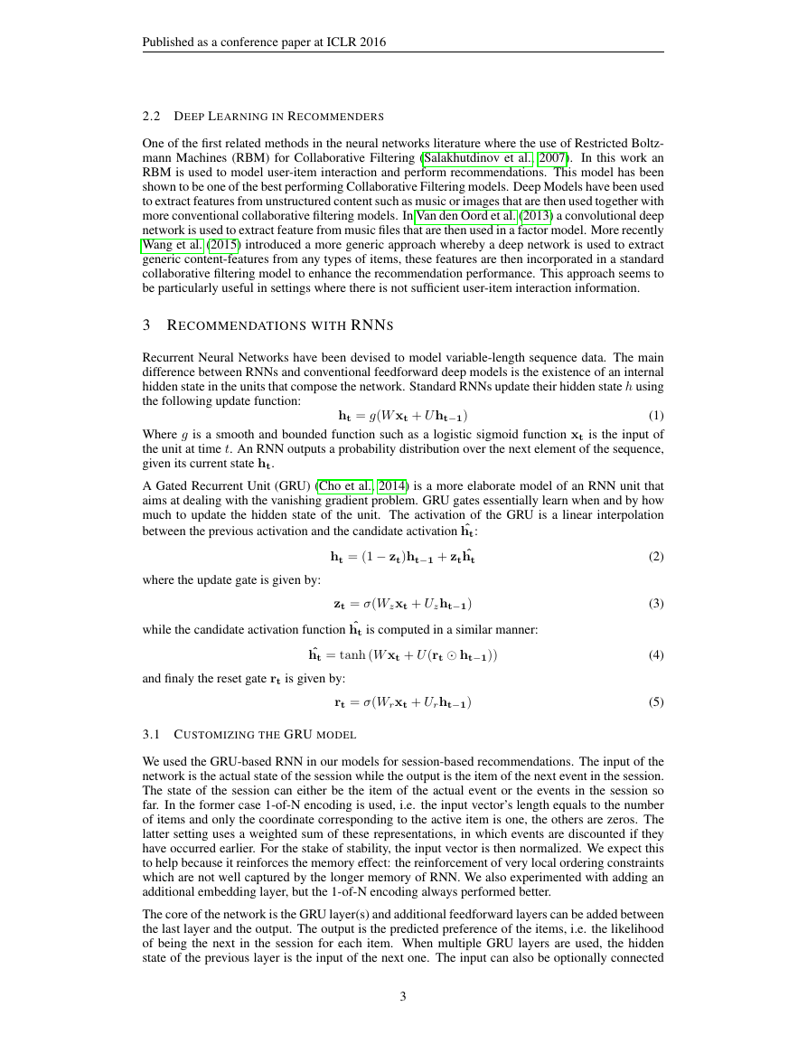
Figure 1: General architecture of the network. Processing of one event of the event stream at once.
to GRU layers deeper in the network, as we found that this improves performance. See the whole
architecture on Figure 1, which depicts the representation of a single event within a time series of
events.
Since recommender systems are not the primary application area of recurrent neural networks, we
modified the base network to better suit the task. We also considered practical points so that our
solution could be possibly applied in a live environment.
3.1.1 SESSION-PARALLEL MINI-BATCHES
RNNs for natural language processing tasks usually use in-sequence mini-batches. For example it
is common to use a sliding window over the words of sentences and put these windowed fragments
next to each other to form mini-batches. This does not fit our task, because (1) the length of sessions
can be very different, even more so than that of sentences: some sessions consist of only 2 events,
while others may range over a few hundreds; (2) our goal is to capture how a session evolves over
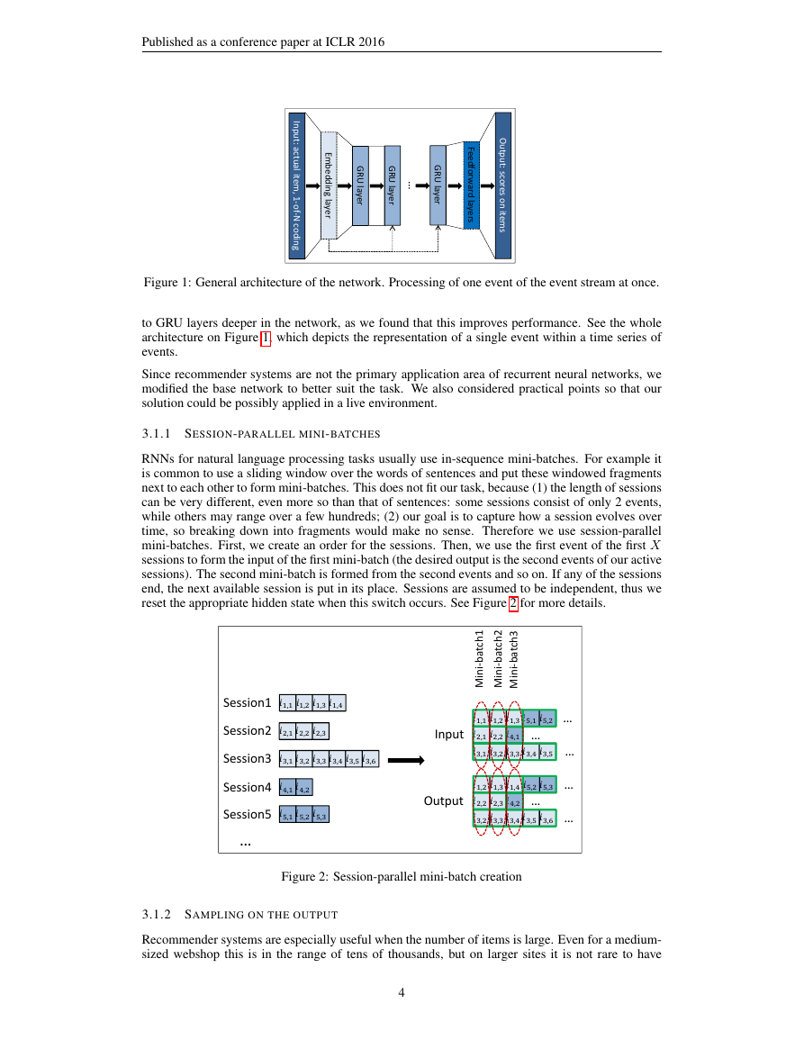
time, so breaking down into fragments would make no sense. Therefore we use session-parallel
mini-batches. First, we create an order for the sessions. Then, we use the first event of the first X
sessions to form the input of the first mini-batch (the desired output is the second events of our active
sessions). The second mini-batch is formed from the second events and so on. If any of the sessions
end, the next available session is put in its place. Sessions are assumed to be independent, thus we
reset the appropriate hidden state when this switch occurs. See Figure 2 for more details.
Figure 2: Session-parallel mini-batch creation
3.1.2 SAMPLING ON THE OUTPUT
Recommender systems are especially useful when the number of items is large. Even for a medium-
sized webshop this is in the range of tens of thousands, but on larger sites it is not rare to have
4
GRU layerFeedforwardlayersGRU layerInput: actualitem, 1-of-N codingEmbeddinglayerGRU layer…Output: scoresonitems,,,,,,,,,,,,,,,,,,Session1Session2Session3Session4Session5…,,,,,,,,,,,,,,,,,,,,,,,,,,InputOutputMini-batch1Mini-batch2Mini-batch3………………�
Published as a conference paper at ICLR 2016
hundreds of thousands of items or even a few millions. Calculating a score for each item in each
step would make the algorithm scale with the product of the number of items and the number of
events. This would be unusable in practice. Therefore we have to sample the output and only
compute the score for a small subset of the items. This also entails that only some of the weights
will be updated. Besides the desired output, we need to compute scores for some negative examples
and modify the weights so that the desired output is highly ranked.
The natural interpretation of an arbitrary missing event is that the user did not know about the
existence of the item and thus there was no interaction. However there is a low probability that
the user did know about the item and chose not to interact, because she disliked the item. The
more popular the item, the more probable it is that the user knows about it, thus it is more likely
that a missing event expresses dislike. Therefore we should sample items in proportion of their
popularity. Instead of generating separate samples for each training example, we use the items from
the other training examples of the mini-batch as negative examples. The benefit of this approach
is that we can further reduce computational times by skipping the sampling. Additionally, there
are also benefits on the implementation side from making the code less complex to faster matrix
operations. Meanwhile, this approach is also a popularity-based sampling, because the likelihood of
an item being in the other training examples of the mini-batch is proportional to its popularity.
3.1.3 RANKING LOSS
The core of recommender systems is the relevance-based ranking of items. Although the task can
also be interpreted as a classification task, learning-to-rank approaches (Rendle et al., 2009; Shi
et al., 2012; Steck, 2015) generally outperform other approaches. Ranking can be pointwise, pair-
wise or listwise. Pointwise ranking estimates the score or the rank of items independently of each
other and the loss is defined in a way so that the rank of relevant items should be low. Pairwise rank-
ing compares the score or the rank of pairs of a positive and a negative item and the loss enforces
that the rank of the positive item should be lower than that of the negative one. Listwise ranking
uses the scores and ranks of all items and compares them to the perfect ordering. As it includes
sorting, it is usually computationally more expensive and thus not used often. Also, if there is only
one relevant item – as in our case – listwise ranking can be solved via pairwise ranking.
We included several pointwise and pairwise ranking losses into our solution. We found that point-
wise ranking was unstable with this network (see Section 4 for more comments). Pairwise ranking
losses on the other hand performed well. We use the following two.
• BPR: Bayesian Personalized Ranking (Rendle et al., 2009) is a matrix factorization method
that uses pairwise ranking loss. It compares the score of a positive and a sampled negative
item. Here we compare the score of the positive item with several sampled items and use
their average as the loss. The loss at a given point in one session is defined as: Ls =
− 1
j=1 log (σ (ˆrs,i − ˆrs,j)), where NS is the sample size, ˆrs,k is the score on item k
at the given point of the session, i is the desired item (next item in the session) and j are
the negative samples.
·NS
NS
·NS
• TOP1: This ranking loss was devised by us for this task. It is the regularized approximation
of the relative rank of the relevant item. The relative rank of the relevant item is given by
j=1 I{ˆrs,j > ˆrs,i}. We approximate I{·} with a sigmoid. Optimizing for this
1
NS
would modify parameters so that the score for i would be high. However this is unstable
as certain positive items also act as negative examples and thus scores tend to become
increasingly higher. To avoid this, we want to force the scores of the negative examples to
be around zero. This is a natural expectation towards the scores of negative items. Thus
we added a regularization term to the loss. It is important that this term is in the same
range as the relative rank and acts similarly to it. The final loss function is as follows:
Ls = 1
NS
j=1 σ (ˆrs,j − ˆrs,i) + σˆr2
·NS
s,j
4 EXPERIMENTS
We evaluate the proposed recursive neural network against popular baselines on two datasets.
5
�
Published as a conference paper at ICLR 2016
The first dataset is that of RecSys Challenge 20151. This dataset contains click-streams of an e-
commerce site that sometimes end in purchase events. We work with the training set of the challenge
and keep only the click events. We filter out sessions of length 1. The network is trained on ∼ 6
months of data, containing 7,966,257 sessions of 31,637,239 clicks on 37,483 items. We use the
sessions of the subsequent day for testing. Each session is assigned to either the training or the test
set, we do not split the data mid-session. Because of the nature of collaborative filtering methods,
we filter out clicks from the test set where the item clicked is not in the train set. Sessions of length
one are also removed from the test set. After the preprocessing we are left with 15,324 sessions of
71,222 events for the test set. This dataset will be referred to as RSC15.
The second dataset is collected from a Youtube-like OTT video service platform. Events of watching
a video for at least a certain amount of time were collected. Only certain regions were subject
to this collection that lasted for somewhat shorter than 2 months. During this time item-to-item
recommendations were provided after each video at the left side of the screen. These were provided
by a selection of different algorithms and influenced the behavior of the users. Preprocessing steps
are similar to that of the other dataset with the addition of filtering out very long sessions as they were
probably generated by bots. The training data consists of all but the last day of the aforementioned
period and has ∼ 3 million sessions of ∼ 13 million watch events on 330 thousand videos. The test
set contains the sessions of the last day of the collection period and has ∼ 37 thousand sessions with
∼ 180 thousand watch events. This dataset will be referred to as VIDEO.
The evaluation is done by providing the events of a session one-by-one and checking the rank of the
item of the next event. The hidden state of the GRU is reset to zero after a session finishes. Items are
ordered in descending order by their score and their position in this list is their rank. With RSC15,
all of the 37,483 items of the train set were ranked. However, this would have been impractical
with VIDEO, due to the large number of items. There we ranked the desired item against the most
popular 30,000 items. This has negligible effect on the evaluations as rarely visited items often get
low scores. Also, popularity based pre-filtering is common in practical recommender systems.
As recommender systems can only recommend a few items at once, the actual item a user might
pick should be amongst the first few items of the list. Therefore, our primary evaluation metric is
recall@20 that is the proportion of cases having the desired item amongst the top-20 items in all test
cases. Recall does not consider the actual rank of the item as long as it is amongst the top-N. This
models certain practical scenarios well where there is no highlighting of recommendations and the
absolute order does not matter. Recall also usually correlates well with important online KPIs, such
as click-through rate (CTR)(Liu et al., 2012; Hidasi & Tikk, 2012). The second metric used in the
experiments is MRR@20 (Mean Reciprocal Rank). That is the average of reciprocal ranks of the
desired items. The reciprocal rank is set to zero if the rank is above 20. MRR takes into account the
rank of the item, which is important in cases where the order of recommendations matter (e.g. the
lower ranked items are only visible after scrolling).
4.1 BASELINES
We compare the proposed network to a set of commonly used baselines.
set. Despite its simplicity it is often a strong baseline in certain domains.
• POP: Popularity predictor that always recommends the most popular items of the training
• S-POP: This baseline recommends the most popular items of the current session. The rec-
ommendation list changes during the session as items gain more events. Ties are broken up
using global popularity values. This baseline is strong in domains with high repetitiveness.
• Item-KNN: Items similar to the actual item are recommended by this baseline and simi-
larity is defined as the cosine similarity between the vector of their sessions, i.e. it is the
number of co-occurrences of two items in sessions divided by the square root of the product
of the numbers of sessions in which the individual items are occurred. Regularization is
also included to avoid coincidental high similarities of rarely visited items. This baseline is
one of the most common item-to-item solutions in practical systems, that provides recom-
mendations in the “others who viewed this item also viewed these ones” setting. Despite
of its simplicity it is usually a strong baseline (Linden et al., 2003; Davidson et al., 2010).
1http://2015.recsyschallenge.com/
6
�
Published as a conference paper at ICLR 2016
Table 1: Recall@20 and MRR@20 using the baseline methods
Baseline
POP
S-POP
Item-KNN
BPR-MF
RSC15
VIDEO
Recall@20 MRR@20 Recall@20 MRR@20
0.0050
0.2672
0.5065
0.2574
0.0012
0.1775
0.2048
0.0618
0.0499
0.1301
0.5508
0.0692
0.0117
0.0863
0.3381
0.0374
Table 2: Best parametrizations for datasets/loss functions
Dataset Loss
TOP1
RSC15
BPR
RSC15
Cross-entropy
RSC15
TOP1
VIDEO
VIDEO
BPR
Cross-entropy
VIDEO
Mini-batch Dropout Learning rate Momentum
50
50
500
50
50
200
0.5
0.2
0
0.4
0.3
0.1
0.01
0.05
0.01
0.05
0.1
0.05
0
0.2
0
0
0
0.3
• BPR-MF: BPR-MF (Rendle et al., 2009) is one of the commonly used matrix factorization
methods. It optimizes for a pairwise ranking objective function (see Section 3) via SGD.
Matrix factorization cannot be applied directly to session-based recommendations, because
the new sessions do not have feature vectors precomputed. However we can overcome this
by using the average of item feature vectors of the items that had occurred in the session
so far as the user feature vector. In other words we average the similarities of the feature
vectors between a recommendable item and the items of the session so far.
Table 1 shows the results for the baselines. The item-KNN approach clearly dominates the other
methods.
4.2 PARAMETER & STRUCTURE OPTIMIZATION
We optimized the hyperparameters by running 100 experiments at randomly selected points of the
parameter space for each dataset and loss function. The best parametrization was further tuned by
individually optimizing each parameter. The number of hidden units was set to 100 in all cases. The
best performing parameters were then used with hidden layers of different sizes. The optimization
was done on a separate validation set. Then the networks were retrained on the training plus the
validation set and evaluated on the final test set.
The best performing parametrizations are summarized in table 2. Weight matrices were initialized
by random numbers drawn uniformly from [−x, x] where x depends on the number of rows and
columns of the matrix. We experimented with both rmsprop (Dauphin et al., 2015) and adagrad
(Duchi et al., 2011). We found adagrad to give better results.
We briefly experimented with other units than GRU. We found both the classic RNN unit and LSTM
to perform worse.
We tried out several loss functions. Pointwise ranking based losses, such as cross-entropy and MRR
optimization (as in Steck (2015)) were usually unstable, even with regularization. For example
cross-entropy yielded only 10 and 6 numerically stable networks of the 100 random runs for RSC15
and VIDEO respectively. We assume that this is due to independently trying to achieve high scores
for the desired items and the negative push is small for the negative samples. On the other hand
pairwise ranking-based losses performed well. We found the ones introduced in Section 3 (BPR and
TOP1) to perform the best.
Several architectures were examined and a single layer of GRU units was found to be the best
performer. Adding addition layers always resulted in worst performance w.r.t. both training loss
and recall and MRR measured on the test set. We assume that this is due to the generally short
7
�
Published as a conference paper at ICLR 2016
Table 3: Recall@20 and MRR@20 for different types of a single layer of GRU, compared to the
best baseline (item-KNN). Best results per dataset are highlighted.
Loss / #Units
RSC15
Recall@20
MRR@20
Recall@20
VIDEO
MRR@20
TOP1 100
BPR 100
Cross-entropy 100
TOP1 1000
BPR 1000
Cross-entropy 1000
0.5853 (+15.55%)
0.6069 (+19.82%)
0.6074 (+19.91%)
0.6206 (+22.53%)
0.6322 (+24.82%)
0.5777 (+14.06%)
0.2305 (+12.58%)
0.2407 (+17.54%)
0.2430 (+18.65%)
0.2693 (+31.49%)
0.2467 (+20.47%)
0.2153 (+5.16%)
0.6141 (+11.50%)
0.5999 (+8.92%)
0.6372 (+15.69%)
0.6624 (+20.27%)
0.6311 (+14.58%)
–
0.3511 (+3.84%)
0.3260 (-3.56%)
0.3720 (+10.04%)
0.3891 (+15.08%)
0.3136 (-7.23%)
–
lifespan of the sessions not requiring multiple time scales of different resolutions to be properly
represented. However the exact reason of this is unknown as of yet and requires further research.
Using embedding of the items gave slightly worse results, therefore we kept the 1-of-N encoding.
Also, putting all previous events of the session on the input instead of the preceding one did not
result in additional accuracy gain; which is not surprising as GRU – like LSTM – has both long and
short term memory. Adding additional feed-forward layers after the GRU layer did not help either.
However increasing the size of the GRU layer improved the performance. We also found that it is
beneficial to use tanh as the activation function of the output layer.
4.3 RESULTS
Table 3 shows the results of the best performing networks. Cross-entropy for the VIDEO data
with 1000 hidden units was numerically unstable and thus we present no results for that scenario.
The results are compared to the best baseline (item-KNN). We show results with 100 and 1000
hidden units. The running time depends on the parameters and the dataset. Generally speaking the
difference in runtime between the smaller and the larger variant is not too high on a GeForce GTX
Titan X GPU and the training of the network can be done in a few hours2. On CPU, the smaller
network can be trained in a practically acceptable timeframe. Frequent retraining is often desirable
for recommender systems, because new users and items are introduced frequently.
The GRU-based approach has substantial gain over the item-KNN in both evaluation metrics on both
datasets, even if the number of units is 1003. Increasing the number of units further improves the
results for pairwise losses, but the accuracy decreases for cross-entropy. Even though cross-entropy
gives better results with 100 hidden units, the pairwise loss variants surpass these results as the
number of units increase. Although, increasing the number of units increases the training times, we
found that it was not too expensive to move from 100 units to 1000 on GPU. Also, the cross-entropy
based loss was found to be numerically unstable as the result of the network individually trying to
increase the score for the target items, while the negative push is relatively small for the other items.
Therefore we suggest using any of the two pairwise losses. The TOP1 loss performs slightly better
on these two datasets, resulting in ∼ 20 − 30% accuracy gain over the best performing baseline.
5 CONCLUSION & FUTURE WORK
In this paper we applied a kind of modern recurrent neural network (GRU) to new application do-
main: recommender systems. We chose the task of session based recommendations, because it is
a practically important area, but not well researched. We modified the basic GRU in order to fit
the task better by introducing session-parallel mini-batches, mini-batch based output sampling and
ranking loss function. We showed that our method can significantly outperform popular baselines
that are used for this task. We think that our work can be the basis of both deep learning applications
in recommender systems and session based recommendations in general.
2Using Theano with fixes for the subtensor operators on GPU.
3Except for using the BPR loss on the VIDEO data and evaluating for MRR.
8
�


 2023年江西萍乡中考道德与法治真题及答案.doc
 2012年重庆南川中考生物真题及答案.doc
 2013年江西师范大学地理学综合及文艺理论基础考研真题.doc
 2020年四川甘孜小升初语文真题及答案I卷.doc
 2020年注册岩土工程师专业基础考试真题及答案.doc
 2023-2024学年福建省厦门市九年级上学期数学月考试题及答案.doc
 2021-2022学年辽宁省沈阳市大东区九年级上学期语文期末试题及答案.doc
 2022-2023学年北京东城区初三第一学期物理期末试卷及答案.doc
 2018上半年江西教师资格初中地理学科知识与教学能力真题及答案.doc
 2012年河北国家公务员申论考试真题及答案-省级.doc
 2020-2021学年江苏省扬州市江都区邵樊片九年级上学期数学第一次质量检测试题及答案.doc
 2022下半年黑龙江教师资格证中学综合素质真题及答案.doc