1
Past, Present, and Future of Simultaneous
Localization And Mapping: Towards the
Robust-Perception Age
Cesar Cadena, Luca Carlone, Henry Carrillo, Yasir Latif,
Davide Scaramuzza, Jos´e Neira, Ian D. Reid, John J. Leonard
6
1
0
2
l
u
J
0
2
]
O
R
.
s
c
[
2
v
0
3
8
5
0
.
6
0
6
1
:
v
i
X
r
a
Abstract—Simultaneous Localization and Mapping (SLAM)
the
consists in the concurrent construction of a model of
environment (the map), and the estimation of the state of the robot
moving within it. The SLAM community has made astonishing
progress over the last 30 years, enabling large-scale real-world
applications, and witnessing a steady transition of this technology
to industry. We survey the current state of SLAM. We start by
presenting what is now the de-facto standard formulation for
SLAM. We then review related work, covering a broad set of
topics including robustness and scalability in long-term mapping,
metric and semantic representations for mapping, theoretical
performance guarantees, active SLAM and exploration, and
other new frontiers. This paper simultaneously serves as a
position paper and tutorial to those who are users of SLAM. By
looking at the published research with a critical eye, we delineate
open challenges and new research issues, that still deserve careful
scientific investigation. The paper also contains the authors’ take
on two questions that often animate discussions during robotics
conferences: Do robots need SLAM? and Is SLAM solved?
Index Terms—Robots, SLAM, localization, mapping.
I. INTRODUCTION
S LAM consists in the simultaneous estimation of the state
of a robot equipped with on-board sensors, and the con-
struction of a model (the map) of the environment that the
sensors are perceiving. In simple instances, the robot state is
described by its pose (position and orientation), although other
quantities may be included in the state, such as robot velocity,
sensor biases, and calibration parameters. The map, on the
other hand, is a representation of aspects of interest (e.g.,
position of landmarks, obstacles) describing the environment
in which the robot operates.
The need to build a map of the environment is twofold.
First, the map is often required to support other tasks; for
instance, a map can inform path planning or provide an
C. Cadena is with the Autonomous Systems Lab, ETH Zurich, Switzerland.
e-mail: cesarc@ethz.ch
L. Carlone is with the Laboratory for Information and Decision Systems,
Massachusetts Institute of Technology, USA. e-mail: lcarlone@mit.edu
H. Carrillo is with the Escuela de Ciencias Exactas e Ingenier´ıa, Universidad
Sergio Arboleda, Colombia. e-mail: henry.carrillo@usa.edu.co
Y. Latif
I.D. Reid
and
Vision,
for
e-mail:
Robotic
yasir.latif@adelaide.edu.au, ian.reid@adelaide.edu.au
J. Neira is with the Departamento de Inform´atica e Ingenier´ıa de Sistemas,
the Australian Center
are with
University
Australia.
Adelaide,
of
Universidad de Zaragoza, Spain. e-mail: jneira@unizar.es
D. Scaramuzza is with the Robotics and Perception Group, University of
Zurich, Switzerland. e-mail: sdavide@ifi.uzh.ch
J.J. Leonard is with Marine Robotics Group, Massachusetts Institute of
Technology, USA. e-mail: jleonard@mit.edu
intuitive visualization for a human operator. Second, the map
allows limiting the error committed in estimating the state of
the robot. In the absence of a map, dead-reckoning would
quickly drift over time; on the other hand, given a map, the
robot can “reset” its localization error by re-visiting known
areas (the so called loop closure). Therefore, SLAM finds
applications in all scenarios in which a prior map is not
available and needs to be built.
In some robotics applications a map of the environment is
known a priori. For instance, a robot operating on a factory
floor can be provided with a manually-built map of artificial
beacons in the environment. Another example is the case in
which the robot has access to GPS data (the GPS satellites
can be considered as moving beacons at known locations).
The popularity of the SLAM problem is connected with the
emergence of indoor applications of mobile robotics. Indoor
operation rules out the use of GPS to bound the localization
error; furthermore, SLAM provides an appealing alternative
to user-built maps, showing that robot operation is possible in
the absence of an ad-hoc localization infrastructure.
A thorough historical review of the first 20 years of the
SLAM problem is given by Durrant-Whyte and Bailey in
two surveys [14, 94]. These mainly cover what we call the
classical age (1986-2004); the classical age saw the intro-
duction of the main probabilistic formulations for SLAM,
including approaches based on Extended Kalman Filters, Rao-
Blackwellised Particle Filters, and maximum likelihood esti-
mation; moreover, it delineated the basic challenges connected
to efficiency and robust data association. Other two excellent
references describing the three main SLAM formulations of
the classical age are the chapter of Thrun and Leonard [299,
chapter 37] and the book of Thrun, Burgard, and Fox [298].
The subsequent period is what we call the algorithmic-analysis
age (2004-2015), and is partially covered by Dissanayake et
al. in [89]. The algorithmic analysis period saw the study
of fundamental properties of SLAM, including observability,
convergence, and consistency. In this period, the key role of
sparsity towards efficient SLAM solvers was also understood,
and the main open-source SLAM libraries were developed.
We review the main SLAM surveys to date in Table I,
observing that most recent surveys only cover specific aspects
or sub-fields of SLAM. The popularity of SLAM in the last 30
years is not surprising if one thinks about the manifold aspects
that SLAM involves. At the lower level (called the front-end
in Section II) SLAM naturally intersects other research fields
�
2
such as computer vision and signal processing; at the higher
level (that we later call the back-end), SLAM is an appealing
mix of geometry, graph theory, optimization, and probabilistic
estimation. Finally, a SLAM expert has to deal with practical
aspects ranging from sensor modeling to system integration.
The present paper gives a broad overview of the current
state of SLAM, and offers the perspective of part of the
community on the open problems and future directions for
the SLAM research. The paper summarizes the outcome of
the workshop “The Problem of Mobile Sensors: Setting future
goals and indicators of progress for SLAM” [40], held during
the Robotics: Science and System (RSS) conference (Rome,
July 2015). Our main focus is on metric and semantic SLAM,
and we refer the reader to the recent survey of Lowry et
al. [198] for a more comprehensive coverage of vision-based
topological SLAM and place recognition.
Before delving into the paper, we provide our take on
two questions that often animate discussions during robotics
conferences.
Do autonomous robots really need SLAM? Answer-
ing this question requires understanding what makes SLAM
unique. SLAM aims at building a globally consistent rep-
resentation of the environment, leveraging both ego-motion
measurements and loop closures. The keyword here is “loop
closure”:
if we sacrifice loop closures, SLAM reduces to
odometry. In early applications, odometry was obtained by
integrating wheel encoders. The pose estimate obtained from
wheel odometry quickly drifts, making the estimate unusable
after few meters [162, Ch. 6]; this was one of the main thrusts
behind the development of SLAM: the observation of external
landmarks is useful to reduce the trajectory drift and possibly
correct it [227]. However, more recent odometry algorithms
are based on visual and inertial information, and have very
small drift (< 0.5% of the trajectory length [109]). Hence the
question becomes legitimate: do we really need SLAM? Our
answer is three-fold.
First of all, we observe that
the SLAM research done
over the last decade was the one producing the visual-inertial
odometry algorithms that currently represent the state of the
art [109, 201]; in this sense visual-inertial navigation (VIN)
is SLAM: VIN can be considered a reduced SLAM system,
in which the loop closure (or place recognition) module is
disabled. More generally, SLAM led to study sensor fusion
under more challenging setups (i.e., no GPS,
low quality
sensors) than previously considered in other literature (e.g.,
inertial navigation in aerospace engineering).
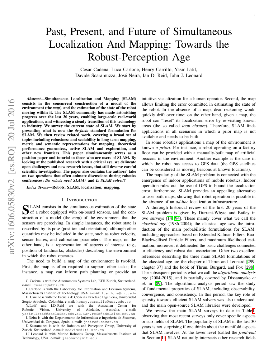
The second answer regards loop closures. A robot perform-
ing odometry and neglecting loop closures interprets the world
as an “infinite corridor” (Fig. 1a) in which the robot keeps
exploring new areas indefinitely. A loop closure event informs
the robot that this “corridor” keeps intersecting itself (Fig. 1b).
The advantage of loop closure now becomes clear: by finding
loop closures, the robot understands the real topology of the
environment, and is able to find shortcuts between locations
(e.g., point B and C in the map). Therefore, if getting the
right topology of the environment is one of the merits of
SLAM, why not simply drop the metric information and
just do place recognition? The answer is simple: the metric
TABLE I: Surveying the surveys
Year Topic
Reference
2006 Probabilistic
and data association
approaches
Durrant-Whyte and Bailey [14, 94]
2008 Filtering approaches
Aulinas et al. [12]
2008 Visual SLAM
Neira et al. (special issue) [220]
2011 SLAM back-end
2011 Observability, consistency
and convergence
Grisetti et al. [129]
Dissanayake et al. [89]
2012 Visual odometry
Scaramuzza and Fraundofer
274]
[115,
2016 Multi robot SLAM
Saeedi et al. [271]
2016 Visual place recognition
Lowry et al. [198]
information makes place recognition much simpler and more
robust; the metric reconstruction informs the robot about loop
closure opportunities and allows discarding spurious loop clo-
sures [187, 295]. Therefore, while SLAM might be redundant
in principle (an oracle place recognition module would suffice
for topological mapping), SLAM offers a natural defense
against wrong data association and perceptual aliasing, where
similarly looking scenes, corresponding to distinct locations
in the environment, would deceive place recognition. In this
sense, the SLAM map provides a way to predict and validate
future measurements: we believe that this mechanism is key
to robust operation.
The third answer is that SLAM is needed since many appli-
cations implicitly or explicitly do require a globally consistent
map. For instance, in many military and civil applications the
goal of the robot is to explore an environment and report
a map to the human operator. Another example is the case
in which the robot has to perform structural inspection (of a
building, bridge, etc.); also in this case a globally consistent
3D reconstruction is a requirement for successful operation.
One can identify tasks for which different flavors of SLAM
formulations are more suitable than others. Therefore, when a
roboticist has to design a SLAM system, he/she is faced with
multiple design choices. For instance, a topological map can
be used to analyze reachability of a given place, but it is not
suitable for motion planning and low-level control; a locally-
consistent metric map is well-suited for obstacle avoidance and
local interactions with the environment, but it may sacrifice
accuracy; a globally-consistent metric map allows the robot to
perform global path planning, but it may be computationally
demanding to compute and maintain. A more general way
to choose the most appropriate SLAM system is to think
about SLAM as a mechanism to compute a sufficient statistic
that summarizes all past observations of the robot, and in
this sense, which information to retain in this compressed
representation is deeply task-dependent.
Is SLAM solved? This is another question that is often
asked within the robotics community, c.f. [118]. The difficulty
of answering this question lies in the question itself: SLAM
is such a broad topic that the question is well posed only
for a given robot/environment/performance combination. In
�
3
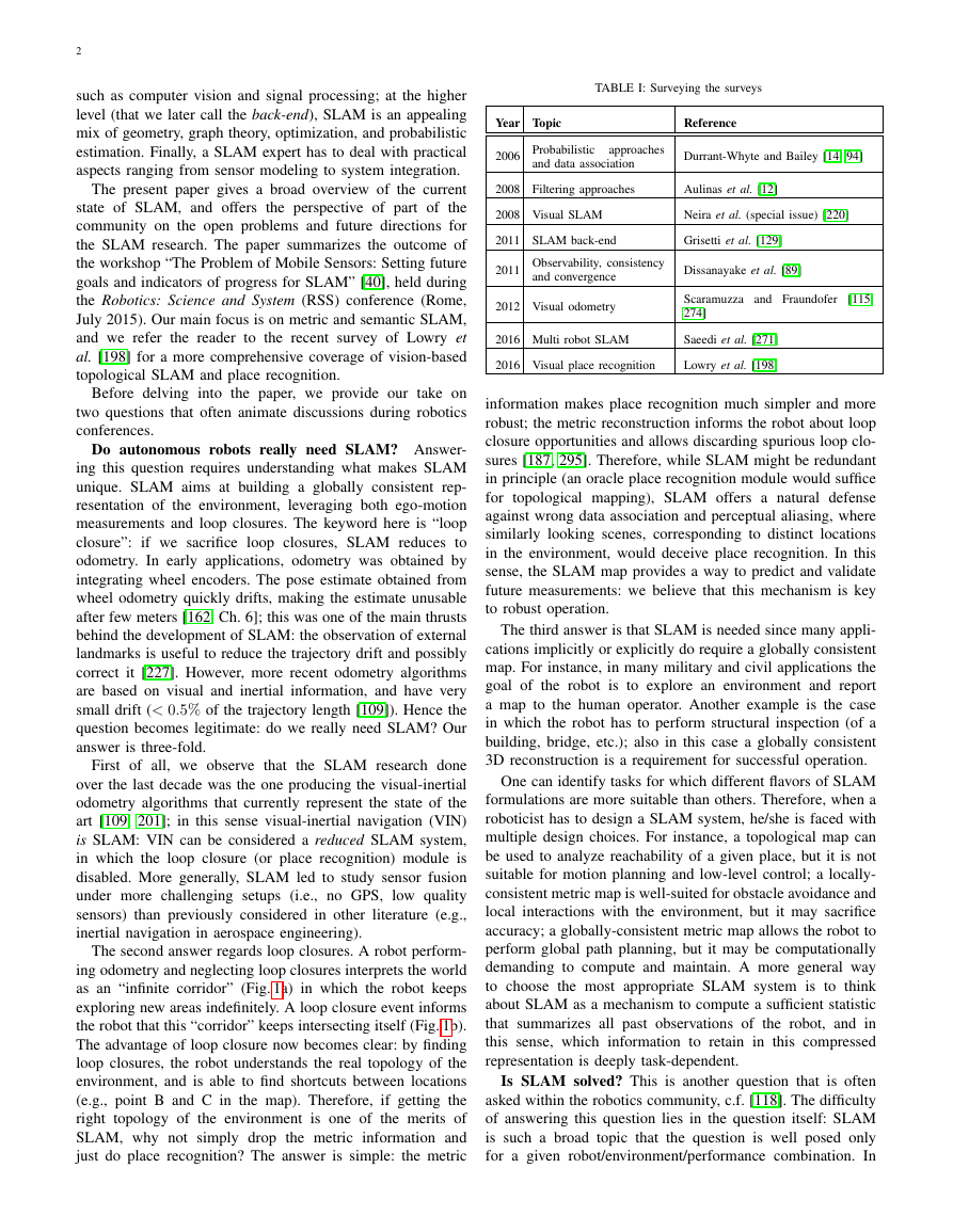
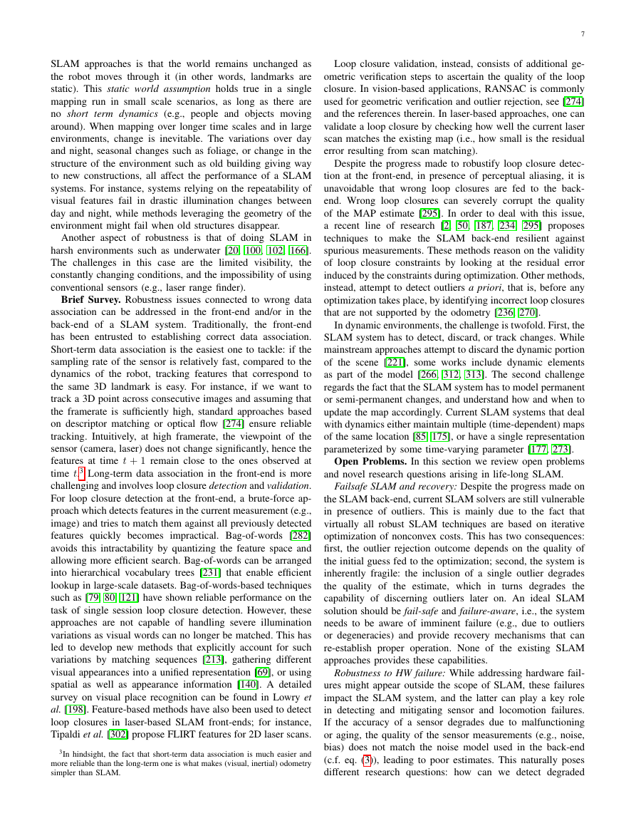
Fig. 2: Front-end and back-end in a typical SLAM system.
and has self-tuning capabilities1 in that it can adapt the
selection of the system parameters to the scenario.
2) high-level understanding: the SLAM system goes be-
yond basic geometry reconstruction to obtain a high-
level understanding of the environment (e.g., semantic,
affordances, high-level geometry, physics);
3) resource awareness:
the SLAM system is tailored to
the available sensing and computational resources, and
provides means to adjust the computation load depending
on the available resources;
4) task-driven inference: the SLAM system produces adap-
tive map representations, whose complexity can change
depending on the task that the robot has to perform.
Paper organization. The paper starts by presenting a
standard formulation and architecture for SLAM (Section II).
Section III tackles robustness in life-long SLAM. Section IV
deals with scalability. Section V discusses how to represent
the geometry of the environment. Section VI extends the
question of the environment representation to the modeling
of semantic information. Section VII provides an overview
of the current accomplishments on the theoretical aspects of
SLAM. Section VIII broadens the discussion and reviews the
active SLAM problem in which decision making is used to
improve the quality of the SLAM results. Section IX provides
an overview of recent trends in SLAM, including the use
of unconventional sensors. Section X provides final remarks.
Throughout the paper, we provide many pointers to related
work outside the robotics community. Despite its unique traits,
SLAM is related to problems addressed in computer vision,
computer graphics, and control theory, and cross-fertilization
among these fields is a necessary condition to enable fast
progress.
For the non-expert reader, we recommend to read Durrant-
Whyte and Bailey’s SLAM tutorials [14, 94] before delving
in this position paper. The more experienced researchers can
jump directly to the section of interest, where they will find
a self-contained overview of the state of the art and open
problems.
II. ANATOMY OF A MODERN SLAM SYSTEM
The architecture of a SLAM system includes two main
components: the front-end and the back-end. The front-end
abstracts sensor data into models that are amenable for
1The SLAM community has been largely affected by the “curse of manual
tuning”, in that satisfactory operation is enabled by expert tuning of the system
parameters (e.g., stopping conditions, thresholds for outlier rejection).
Fig. 1: Left: map built from odometry. The map is homotopic to a long corridor
that goes from the starting position A to the final position B. Points that are
close in reality (e.g., B and C) may be arbitrarily far in the odometric map.
Right: map build from SLAM. By leveraging loop closures, SLAM estimates
the actual topology of the environment, and “discovers” shortcuts in the map.
particular, one can evaluate the maturity of the SLAM problem
once the following aspects are specified:
• robot: type of motion (e.g., dynamics, maximum speed),
available sensors (e.g., resolution, sampling rate), avail-
able computational resources;
• environment: planar or three-dimensional, presence of
natural or artificial landmarks, amount of dynamic ele-
ments, amount of symmetry and risk of perceptual alias-
ing. Note that many of these aspects actually depend on
the sensor-environment pair: for instance, two rooms may
look identical for a 2D laser scanner (perceptual aliasing),
while a camera may discern them from appearance cues;
• performance requirements: desired accuracy in the esti-
mation of the state of the robot, accuracy and type of
representation of the environment (e.g., landmark-based
or dense), success rate (percentage of tests in which the
accuracy bounds are met), estimation latency, maximum
operation time, maximum size of the mapped area.
For instance, mapping a 2D indoor environment with a
robot equipped with wheel encoders and a laser scanner,
with sufficient accuracy (< 10cm ) and sufficient robustness
(say, low failure rate), can be considered largely solved (an
example of industrial system performing SLAM is the Kuka
Navigation Solution [182]). Similarly, vision-based SLAM
with slowly-moving robots (e.g., Mars rovers [203], domes-
tic robots [148]), and visual-inertial odometry [126] can be
considered mature research fields. On the other hand, other
robot/environment/performance combinations still deserve a
large amount of fundamental research. Current SLAM algo-
rithms can be easily induced to fail when either the motion
of the robot or the environment are too challenging (e.g.,
fast robot dynamics, highly dynamic environments); similarly,
SLAM algorithms are often unable to face strict performance
requirements, e.g., high rate estimation for fast closed-loop
control. This survey will provide a comprehensive overview
of these open problems, among others.
We conclude this section with some broader considerations
about the future of SLAM. We argue that we are entering
in a third era for SLAM, the robust-perception age, which is
characterized by the following key requirements:
1) robust performance: the SLAM system operates with low
failure rate for an extended period of time in a broad set of
environments; the system includes fail-safe mechanisms
�
4
estimation, while the back-end performs inference on the
abstracted data produced by the front-end. This architecture
is summarized in Fig. 2. We review both components, starting
from the back-end.
Maximum-a-posteriori (MAP) estimation and the SLAM
back-end. The current de-facto standard formulation of SLAM
has its origins in the seminal paper of Lu and Milios [199],
followed by the work of Gutmann and Konolige [133]. Since
then, numerous approaches have improved the efficiency and
robustness of the optimization underlying the problem [88,
108, 132, 159, 160, 235, 301]. All these approaches formulate
SLAM as a maximum-a-posteriori estimation problem, and
often use the formalism of factor graphs [180] to reason about
the interdependence among variables.
Assume that we want to estimate an unknown variable X ; as
mentioned before, in SLAM the variable X typically includes
the trajectory of the robot (as a discrete set of poses) and
the position of landmarks in the environment. We are given
a set of measurements Z = {zk : k = 1, . . . , m} such that
each measurement can be expressed as a function of X , i.e.,
zk = hk(Xk) + �k, where Xk ⊆ X is a subset of the variables,
hk(·) is a known function (the measurement or observation
model), and �k is random measurement noise.
In MAP estimation, we estimate X by computing the
assignment of variables X that attains the maximum of the
posterior p(X|Z) (the belief over X given the measurements):
X .
= argmax
X
p(X|Z) = argmax
X
p(Z|X )p(X )
(1)
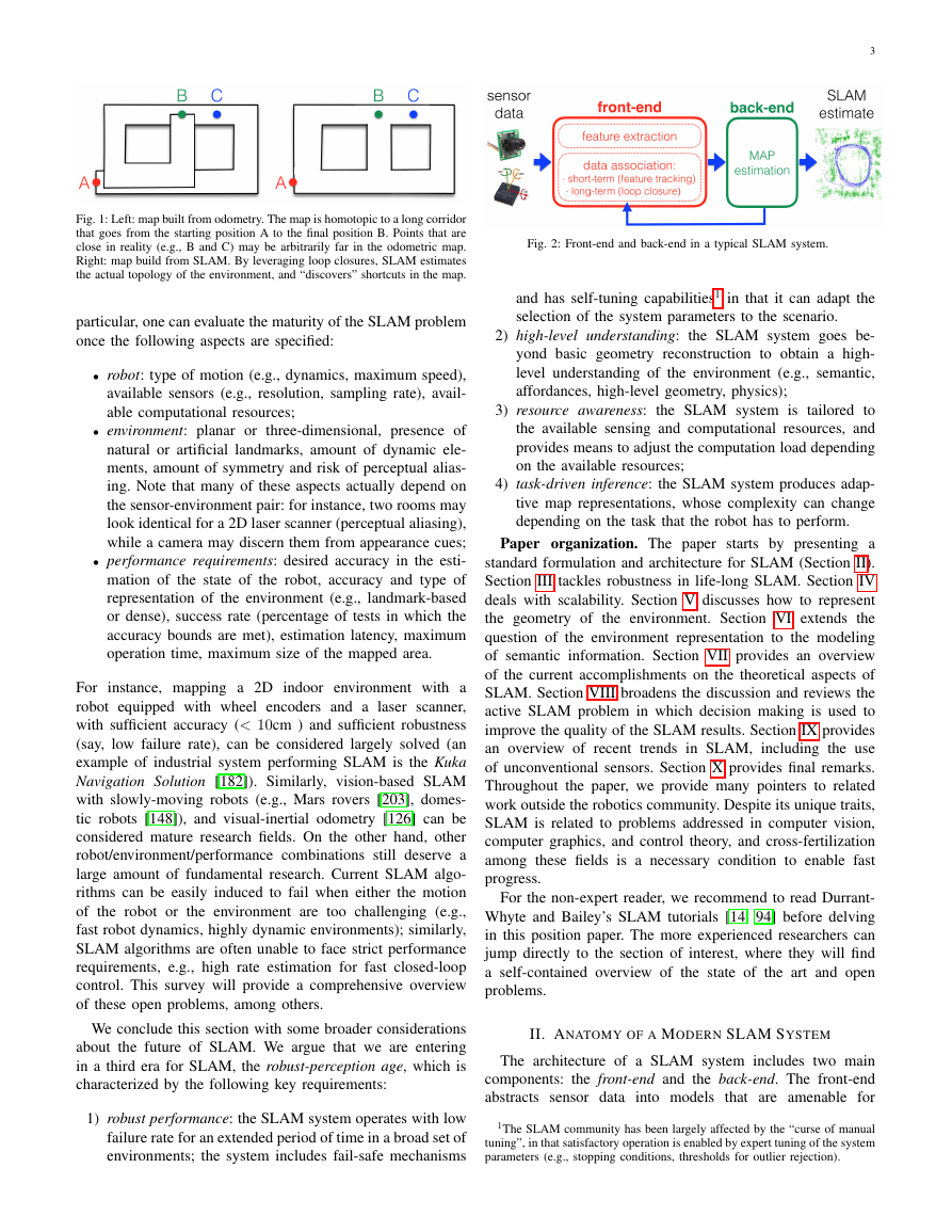
Fig. 3: SLAM as a factor graph: Blue circles denote robot poses at
consecutive time steps (x1, x2, . . .), green circles denote landmark positions
(l1, l2, . . .), red circle denotes the variable associated with the intrinsic
calibration parameters (K). Factors are shows are black dots:
the label
“u” marks factors corresponding to odometry constraints, “v” marks factors
corresponding to camera observations, “c” denotes loop closures, and “p”
denotes prior factors.
among these variables. A second advantage is generality: a
factor graph can model complex inference problems with
heterogeneous variables and factors, and arbitrary interconnec-
tions; the connectivity of the factor graph in turns influences
the sparsity of the resulting SLAM problem as discussed
below.
In order to write (2) in a more explicit form, assume that
the measurement noise �k is a zero-mean Gaussian noise with
information matrix Ωk (inverse of the covariance matrix).
Then, the measurement likelihood in (2) becomes:
where the equality follows from the Bayes theorem. In (1),
p(Z|X ) is the likelihood of the measurements Z given the
assignment X , and p(X ) is a prior probability over X . The
prior probability includes any prior knowledge about X ; in
case no prior knowledge is available, p(X ) becomes a constant
(uniform distribution) which is inconsequential and can be
dropped from the optimization. In that case MAP estimation
reduces to maximum likelihood estimation.
Assuming that the measurements Z are independent (i.e.,
the noise terms affecting the measurements are not correlated),
problem (1) factorizes into:
X = argmax
p(zk|X ) = p(X )
p(zk|Xk) (2)
m
m
p(X )
X
k=1
k=1
where, on the right-hand-side, we noticed that zk only depends
on the subset of variables in Xk.
Problem (2) can be interpreted in terms of inference over a
factors graph [180]. The variables correspond to nodes in the
factor graph. The terms p(zk|Xk) and the prior p(X ) are called
factors, and they encode probabilistic constraints over a subset
of nodes. A factor graph is a graphical model that encodes
the dependence between the k-th factor (and its measurement
zk) and the corresponding variables Xk. A first advantage of
the factor graph interpretation is that it enables an insightful
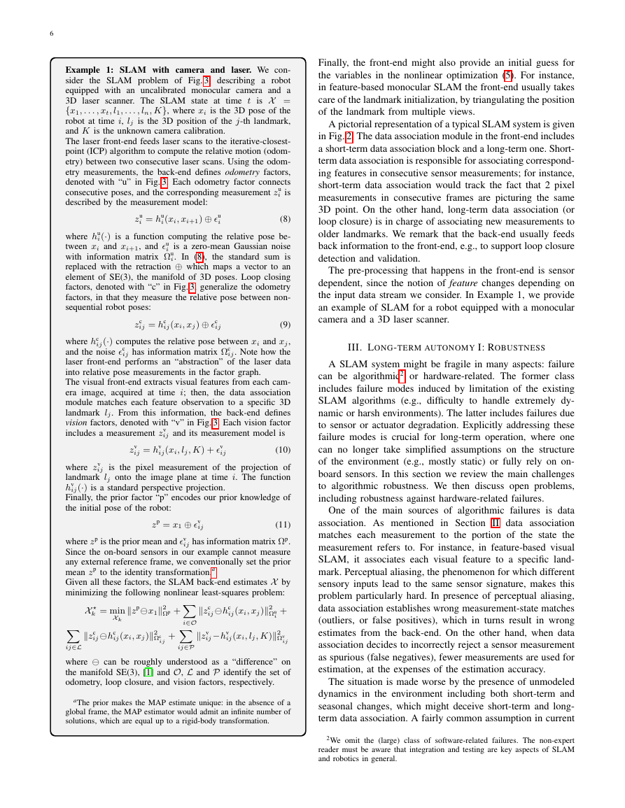
visualization of the problem. Fig. 3 shows an example of factor
graph underlying a simple SLAM problem (more details in
Example 1 below). The figure shows the variables, namely,
the robot poses,
the landmarks positions, and the camera
calibration parameters, and the factors imposing constraints
p(zk|Xk) ∝ exp(− 1
2
where we use the notation ||e||2
that the prior can be written as:
p(X ) ∝ exp(− 1
2
||hk(Xk) − zk||2
Ωk
)
(3)
Ω = eTΩe. Similarly, assume
||h0(X ) − z0||2
(4)
for some given function h0(·), prior mean z0, and information
matrix Ω0. Since maximizing the posterior is the same as
minimizing the negative log-posterior,
the MAP estimate
in (2) becomes:
Ω0
)
X = argmin
X
−log
m
p(X )
m
k=0
argmin
X
p(zk|Xk)
=
k=1
||hk(Xk) − zk||2
Ωk
(5)
which is a nonlinear least squares problem, as in most prob-
lems of interest in robotics, hk(·) is a nonlinear function.
Note that the formulation (5) follows from the assumption of
Normally distributed noise. Other assumptions for the noise
distribution lead to different cost functions; for instance, if the
noise follows a Laplace distribution, the squared 2-norm in (5)
is replaced by the 1-norm. To increase resilience to outliers, it
is also common to substitute the squared 2-norm in (5) with
robust loss functions (e.g., Huber or Tukey loss) [146].
The computer vision expert may notice a resemblance
between problem (5) and bundle adjustment (BA) in Structure
from Motion [305]; both (5) and BA indeed stem from a
�
to mention a few. For instance,
maximum-a-posteriori formulation. However, two key features
make SLAM unique. First, the factors in (5) are not con-
strained to model projective geometry as in BA, but include a
broad variety of sensor models, e.g., inertial sensors, wheel
encoders, GPS,
in laser-
based mapping, the factors usually constrain relative poses
corresponding to different viewpoints, while in direct methods
for visual SLAM, the factors penalize differences in pixel
intensities across different views of the same portion of the
scene. The second difference with respect to BA is that prob-
lem (5) needs to be solved incrementally: new measurements
are made available at each time step as the robot moves.
The minimization problem (5) is commonly solved via
successive linearizations, e.g.,
the Gauss-Newton (GN) or
the Levenberg-Marquardt methods (more modern approaches,
based on convex relaxations and Lagrangian duality are re-
viewed in Section VII). The Gauss-Newton method proceeds
iteratively, starting from a given initial guess ˆX . At each
iteration, GN approximates the minimization (5) as
m
Ωk
Ω
δX
δX
k=0
= argmin
δX = argmin
||Ak δX − bk||2
||A δX − b||2
(6)
where δX is a small “correction” with respect to the lineariza-
tion point ˆX , Ak
is the Jacobian of the measurement
function hk(·) with respect to X , bk
= zk − hk( ˆXk) is the
.
residual error at ˆX ; on the right-hand-side of (6), A (resp. b)
is obtained by stacking Ak (resp. bk); Ωk is a block diagonal
matrix including the measurement information matrices Ωk as
diagonal blocks.
= ∂hk(X )
.
∂X
The optimal correction δX which minimizes (6) can be
computed in closed form as:
δX = (ATΩA)−1ATΩb
(7)
and, at each iteration, the linearization point is updated via
ˆX ← ˆX + δX . The matrix (ATΩA) is usually referred to
as the (approximate) Hessian. Note that this matrix is indeed
only an approximation of the Hessian of the cost function (5);
moreover, its invertibility is connected to the observability
properties of the underlying estimation problem.
So far we assumed that X belongs to a vector space (for
this reason the sum ˆX +δX is well defined). When X includes
variables belonging to a smooth manifold (e.g., rotations), the
structure of the GN method remains unaltered, but the usual
sum (e.g., ˆX + δX ) is substituted with a suitable mapping,
called retraction [1]. In the robotics literature, the retraction
is often denoted with the operator ⊕ and maps the “small
correction” δX defined in the tangent space of the manifold at
ˆX , to an element of the manifold, i.e., the linearization point
is updated as ˆX ← ˆX ⊕ δX . We also note that the derivation
presented so far can be extended to the case in which the
noise is not additive, as long as the noise can be written as an
explicit function of the state and the measurements.
The key insight behind modern SLAM solvers is that the
Jacobian matrix A appearing in (7) is sparse and its sparsity
structure is dictated by the topology of the underlying factor
graph. This enables the use of fast linear solvers to compute
5
δX [159, 160, 183, 252]. Moreover, it allows designing in-
cremental (or online) solvers, which update the estimate of
X as new observations are acquired [159, 160, 252]. Current
SLAM libraries (e.g., GTSAM [86], g2o [183], Ceres [269],
iSAM [160], and SLAM++ [252]) are able to solve problems
with tens of thousands of variables in few seconds. The hands-
on tutorials [86, 129] provide excellent introductions to two of
the most popular SLAM libraries; each library also includes
a set of examples showcasing real SLAM problems.
The SLAM formulation described so far is commonly
referred to as maximum-a-posteriori estimation, factor graph
optimization, graph-SLAM, full smoothing, or smoothing and
mapping (SAM). A popular variation of this framework is pose
graph optimization, in which the variables to be estimated are
poses sampled along the trajectory of the robot, and each factor
imposes a constraint on a pair of poses.
MAP estimation has been proven to be more accurate
and efficient than original approaches for SLAM based on
nonlinear filtering. We refer the reader to the surveys [14, 94]
for an overview on filtering approaches, and to [291] for a
comparison between filtering and smoothing. However, we
remark that some SLAM systems based on EKF have also
been demonstrated to attain state-of-the-art performance. Ex-
cellent examples of EKF-based SLAM systems include the
Multi-State Constraint Kalman Filter of Mourikis and Roume-
liotis [214], and the VIN systems of Kottas et al. [176] and
Hesch et al. [139]. Not surprisingly, the performance mismatch
between filtering and MAP estimation gets smaller when the
linearization point for the EKF is accurate (as it happens
in visual-inertial navigation problems), when using sliding-
window filters, and when potential sources of inconsistency in
the EKF are taken care of [139, 143, 176].
As discussed in the next section, MAP estimation is usually
performed on a pre-processed version of the sensor data. In
this regard, it is often referred to as the SLAM back-end.
Sensor-dependent SLAM front-end. In practical robotics
applications, it might be hard to write directly the sensor
measurements as an analytic function of the state, as required
in MAP estimation. For instance, if the raw sensor data is an
image, it might be hard to express the intensity of each pixel
as a function of the SLAM state; the same difficulty arises
with simpler sensors (e.g., a laser with a single beam). In both
cases the issue is connected with the fact that we are not able to
design a sufficiently general, yet tractable representation of the
environment; even in presence of such general representation,
it would be hard to write an analytic function that connects
the measurements to the parameters of such representation.
For this reason, before the SLAM back-end, it is common
to have a module, the front-end, that extracts relevant features
from the sensor data. For instance, in vision-based SLAM,
the front-end extracts the pixel location of few distinguishable
points in the environment; pixel observations of these points
are now easy to model within the back-end (see Example 1).
The front-end is also in charge of associating each measure-
ment to a specific landmark (say, 3D point) in the environment:
this is the so called data association. More abstractly, the data
association module associates each measurement zk with a
subset of unknown variables Xk such that zk = hk(Xk) + �k.
�
6
Example 1: SLAM with camera and laser. We con-
sider the SLAM problem of Fig. 3, describing a robot
equipped with an uncalibrated monocular camera and a
time t is X =
3D laser scanner. The SLAM state at
{x1, . . . , xt, l1, . . . , ln, K}, where xi is the 3D pose of the
robot at time i, lj is the 3D position of the j-th landmark,
and K is the unknown camera calibration.
The laser front-end feeds laser scans to the iterative-closest-
point (ICP) algorithm to compute the relative motion (odom-
etry) between two consecutive laser scans. Using the odom-
etry measurements, the back-end defines odometry factors,
denoted with “u” in Fig. 3. Each odometry factor connects
consecutive poses, and the corresponding measurement zu
i is
described by the measurement model:
i
i(xi, xi+1) ⊕ �u
zu
i = hu
(8)
i(·) is a function computing the relative pose be-
where hu
tween xi and xi+1, and �u
i is a zero-mean Gaussian noise
with information matrix Ωu
i. In (8), the standard sum is
replaced with the retraction ⊕ which maps a vector to an
element of SE(3), the manifold of 3D poses. Loop closing
factors, denoted with “c” in Fig. 3, generalize the odometry
factors, in that they measure the relative pose between non-
sequential robot poses:
ij
ij(xi, xj) ⊕ �c
zc
ij = hc
ij has information matrix Ωc
(9)
ij(·) computes the relative pose between xi and xj,
where hc
and the noise �c
ij. Note how the
laser front-end performs an “abstraction” of the laser data
into relative pose measurements in the factor graph.
The visual front-end extracts visual features from each cam-
era image, acquired at time i; then, the data association
module matches each feature observation to a specific 3D
landmark lj. From this information, the back-end defines
vision factors, denoted with “v” in Fig. 3. Each vision factor
includes a measurement zv
ij and its measurement model is
ij(xi, lj, K) + �v
zv
ij = hv
(10)
where zv
ij is the pixel measurement of the projection of
landmark lj onto the image plane at time i. The function
ij(·) is a standard perspective projection.
hv
Finally, the prior factor “p” encodes our prior knowledge of
the initial pose of the robot:
ij
zp = x1 ⊕ �v
ij
(11)
where zp is the prior mean and �v
ij has information matrix Ωp.
Since the on-board sensors in our example cannot measure
any external reference frame, we conventionally set the prior
mean zp to the identity transformation.a
Given all these factors, the SLAM back-end estimates X by
minimizing the following nonlinear least-squares problem:
i∈O
X
k = minXk
ijhc
zc
zpx12
Ωp +
ij(xi, xj)2
+
Ωc
ij
zc
ijhc
ij−hv
ij(xi, xj)2
ij(xi, lj, K)2
Ωu
i
zv
+
Ωv
ij
ij∈L
where can be roughly understood as a “difference” on
the manifold SE(3), [1] and O, L and P identify the set of
odometry, loop closure, and vision factors, respectively.
ij∈P
aThe prior makes the MAP estimate unique: in the absence of a
global frame, the MAP estimator would admit an infinite number of
solutions, which are equal up to a rigid-body transformation.
Finally, the front-end might also provide an initial guess for
the variables in the nonlinear optimization (5). For instance,
in feature-based monocular SLAM the front-end usually takes
care of the landmark initialization, by triangulating the position
of the landmark from multiple views.
A pictorial representation of a typical SLAM system is given
in Fig. 2. The data association module in the front-end includes
a short-term data association block and a long-term one. Short-
term data association is responsible for associating correspond-
ing features in consecutive sensor measurements; for instance,
short-term data association would track the fact that 2 pixel
measurements in consecutive frames are picturing the same
3D point. On the other hand, long-term data association (or
loop closure) is in charge of associating new measurements to
older landmarks. We remark that the back-end usually feeds
back information to the front-end, e.g., to support loop closure
detection and validation.
The pre-processing that happens in the front-end is sensor
dependent, since the notion of feature changes depending on
the input data stream we consider. In Example 1, we provide
an example of SLAM for a robot equipped with a monocular
camera and a 3D laser scanner.
III. LONG-TERM AUTONOMY I: ROBUSTNESS
A SLAM system might be fragile in many aspects: failure
can be algorithmic2 or hardware-related. The former class
includes failure modes induced by limitation of the existing
SLAM algorithms (e.g., difficulty to handle extremely dy-
namic or harsh environments). The latter includes failures due
to sensor or actuator degradation. Explicitly addressing these
failure modes is crucial for long-term operation, where one
can no longer take simplified assumptions on the structure
of the environment (e.g., mostly static) or fully rely on on-
board sensors. In this section we review the main challenges
to algorithmic robustness. We then discuss open problems,
including robustness against hardware-related failures.
One of the main sources of algorithmic failures is data
association. As mentioned in Section II data association
matches each measurement to the portion of the state the
measurement refers to. For instance, in feature-based visual
SLAM, it associates each visual feature to a specific land-
mark. Perceptual aliasing, the phenomenon for which different
sensory inputs lead to the same sensor signature, makes this
problem particularly hard. In presence of perceptual aliasing,
data association establishes wrong measurement-state matches
(outliers, or false positives), which in turns result in wrong
estimates from the back-end. On the other hand, when data
association decides to incorrectly reject a sensor measurement
as spurious (false negatives), fewer measurements are used for
estimation, at the expenses of the estimation accuracy.
The situation is made worse by the presence of unmodeled
dynamics in the environment including both short-term and
seasonal changes, which might deceive short-term and long-
term data association. A fairly common assumption in current
2We omit the (large) class of software-related failures. The non-expert
reader must be aware that integration and testing are key aspects of SLAM
and robotics in general.
�
SLAM approaches is that the world remains unchanged as
the robot moves through it (in other words, landmarks are
static). This static world assumption holds true in a single
mapping run in small scale scenarios, as long as there are
no short
term dynamics (e.g., people and objects moving
around). When mapping over longer time scales and in large
environments, change is inevitable. The variations over day
and night, seasonal changes such as foliage, or change in the
structure of the environment such as old building giving way
to new constructions, all affect the performance of a SLAM
systems. For instance, systems relying on the repeatability of
visual features fail in drastic illumination changes between
day and night, while methods leveraging the geometry of the
environment might fail when old structures disappear.
Another aspect of robustness is that of doing SLAM in
harsh environments such as underwater [20, 100, 102, 166].
The challenges in this case are the limited visibility,
the
constantly changing conditions, and the impossibility of using
conventional sensors (e.g., laser range finder).
Brief Survey. Robustness issues connected to wrong data
association can be addressed in the front-end and/or in the
back-end of a SLAM system. Traditionally,
the front-end
has been entrusted to establishing correct data association.
Short-term data association is the easiest one to tackle: if the
sampling rate of the sensor is relatively fast, compared to the
dynamics of the robot, tracking features that correspond to
the same 3D landmark is easy. For instance, if we want to
track a 3D point across consecutive images and assuming that
the framerate is sufficiently high, standard approaches based
on descriptor matching or optical flow [274] ensure reliable
tracking. Intuitively, at high framerate, the viewpoint of the
sensor (camera, laser) does not change significantly, hence the
features at time t + 1 remain close to the ones observed at
time t.3 Long-term data association in the front-end is more
challenging and involves loop closure detection and validation.
For loop closure detection at the front-end, a brute-force ap-
proach which detects features in the current measurement (e.g.,
image) and tries to match them against all previously detected
features quickly becomes impractical. Bag-of-words [282]
avoids this intractability by quantizing the feature space and
allowing more efficient search. Bag-of-words can be arranged
into hierarchical vocabulary trees [231] that enable efficient
lookup in large-scale datasets. Bag-of-words-based techniques
such as [79, 80, 121] have shown reliable performance on the
task of single session loop closure detection. However, these
approaches are not capable of handling severe illumination
variations as visual words can no longer be matched. This has
led to develop new methods that explicitly account for such
variations by matching sequences [213], gathering different
visual appearances into a unified representation [69], or using
spatial as well as appearance information [140]. A detailed
survey on visual place recognition can be found in Lowry et
al. [198]. Feature-based methods have also been used to detect
loop closures in laser-based SLAM front-ends; for instance,
Tipaldi et al. [302] propose FLIRT features for 2D laser scans.
3In hindsight, the fact that short-term data association is much easier and
more reliable than the long-term one is what makes (visual, inertial) odometry
simpler than SLAM.
7
Loop closure validation, instead, consists of additional ge-
ometric verification steps to ascertain the quality of the loop
closure. In vision-based applications, RANSAC is commonly
used for geometric verification and outlier rejection, see [274]
and the references therein. In laser-based approaches, one can
validate a loop closure by checking how well the current laser
scan matches the existing map (i.e., how small is the residual
error resulting from scan matching).
Despite the progress made to robustify loop closure detec-
tion at the front-end, in presence of perceptual aliasing, it is
unavoidable that wrong loop closures are fed to the back-
end. Wrong loop closures can severely corrupt the quality
of the MAP estimate [295]. In order to deal with this issue,
a recent line of research [2, 50, 187, 234, 295] proposes
techniques to make the SLAM back-end resilient against
spurious measurements. These methods reason on the validity
of loop closure constraints by looking at the residual error
induced by the constraints during optimization. Other methods,
instead, attempt to detect outliers a priori, that is, before any
optimization takes place, by identifying incorrect loop closures
that are not supported by the odometry [236, 270].
In dynamic environments, the challenge is twofold. First, the
SLAM system has to detect, discard, or track changes. While
mainstream approaches attempt to discard the dynamic portion
of the scene [221], some works include dynamic elements
as part of the model [266, 312, 313]. The second challenge
regards the fact that the SLAM system has to model permanent
or semi-permanent changes, and understand how and when to
update the map accordingly. Current SLAM systems that deal
with dynamics either maintain multiple (time-dependent) maps
of the same location [85, 175], or have a single representation
parameterized by some time-varying parameter [177, 273].
Open Problems. In this section we review open problems
and novel research questions arising in life-long SLAM.
Failsafe SLAM and recovery: Despite the progress made on
the SLAM back-end, current SLAM solvers are still vulnerable
in presence of outliers. This is mainly due to the fact that
virtually all robust SLAM techniques are based on iterative
optimization of nonconvex costs. This has two consequences:
first, the outlier rejection outcome depends on the quality of
the initial guess fed to the optimization; second, the system is
inherently fragile: the inclusion of a single outlier degrades
the quality of the estimate, which in turns degrades the
capability of discerning outliers later on. An ideal SLAM
solution should be fail-safe and failure-aware, i.e., the system
needs to be aware of imminent failure (e.g., due to outliers
or degeneracies) and provide recovery mechanisms that can
re-establish proper operation. None of the existing SLAM
approaches provides these capabilities.
Robustness to HW failure: While addressing hardware fail-
ures might appear outside the scope of SLAM, these failures
impact the SLAM system, and the latter can play a key role
in detecting and mitigating sensor and locomotion failures.
If the accuracy of a sensor degrades due to malfunctioning
or aging, the quality of the sensor measurements (e.g., noise,
bias) does not match the noise model used in the back-end
(c.f. eq. (3)), leading to poor estimates. This naturally poses
different research questions: how can we detect degraded
�
8
sensor operation? how can we adjust sensor noise statistics
(covariances, biases) accordingly?
Metric Relocalization: While appearance-based, as opposed
to feature-based, methods are able to close loops between day
and night sequences [69, 213], or between different seasons
[223] the resulting loop closure is topological in nature. For
metric relocalization (i.e., estimating the relative pose with
respect to the previously built map), feature-based approaches
are still the norm [121] but have not been extended to such
circumstances. While vision has become the sensor of choice
for many applications and loop closing has become a sensor
signature matching problem [79, 80, 121, 302], other sensors
as well as information inherent to the SLAM problem might
be exploited. For instance, Brubaker et al. [37] use trajectory
matching to address the shortcomings of cameras. Additionally
mapping with one sensor modality and localizing in the same
map with a different sensor modality can be a useful addition.
The work of Wolcott et al. [328] and Forster et al. [111] is
a step in this direction. Another problem is localizing from
significantly different viewpoints with heterogeneous sensing.
Forster et al. [111] study vision-based localization in a lidar-
based map. Majdik et al. [204] study how to localize a drone
in a cadastral 3D model textured from Google Street View
images, Behzadin et al. [21] show how to localize in hand-
drawn maps using a laser scanner, and Winterhalter et al. [327]
carry out RGB-D localization given 2D floor plans.
Time varying and deformable maps: Mainstream SLAM
methods have been developed with the rigid and static world
assumption in mind; however, the real world is non rigid
both due to dynamics as well as the inherent deformability
of objects. An ideal SLAM solution should be able to reason
about dynamics in the environment
including non-rigidity,
work over long time period generating “all
terrain” maps
and be able to do so in real time. In the computer vision
community, there have been several attempts since the 80s
to recover shape from non-rigid objects but with restrictive
applicability, for example Pentland et al. [245, 246] require
prior knowledge of some mechanical properties of the objects,
Bregler et al. in [36] and [304] requires a restricted deforma-
tion of the object and show examples in human faces. Recent
results in non-rigid SfM such as [4, 5, 128] are less restrictive
but still work in small scenarios. In the SLAM community,
Newcombe et al. [225] have address the non-rigid case for
small-scale reconstruction. However, addressing the problem
of non-rigid maps at a large scale is still largely unexplored.
Automatic parameter tuning: SLAM systems (in particular,
the data association modules) require extensive parameter
tuning in order to work correctly for a given scenario. These
parameters include thresholds that control feature matching,
RANSAC parameters, and criteria to decide when to add new
factors to the graph or when to trigger a loop closing algorithm
to search for matches. If SLAM has to work “out of the box”
in arbitrary scenarios, methods for automatic tuning of the
involved parameters need to be considered.
IV. LONG-TERM AUTONOMY II: SCALABILITY
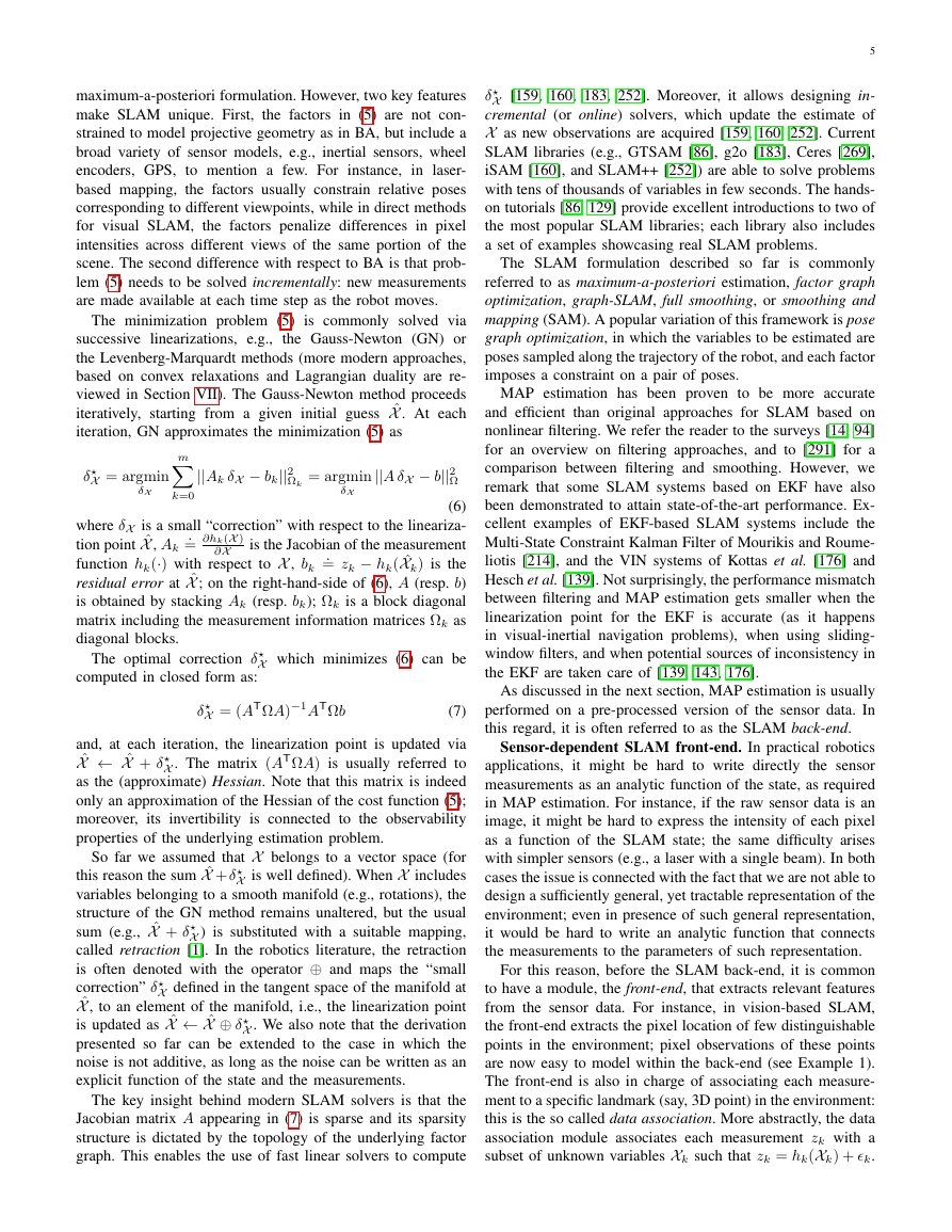
While modern SLAM algorithms have been successfully
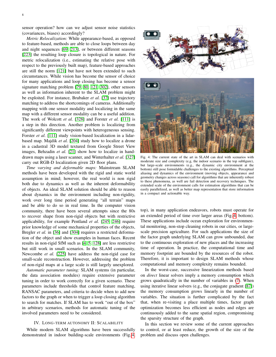
demonstrated in indoor building-scale environments (Fig. 4,
large-scale environments (e.g.,
the dynamic city environment at
Fig. 4: The current state of the art in SLAM can deal with scenarios with
moderate size and complexity (e.g, the indoor scenario in the top subfigure),
but
the
bottom) still pose formidable challenges to the existing algorithms. Perceptual
aliasing and dynamics of the environment (moving objects, appearance and
geometry changes across seasons) call for algorithms that are inherently robust
to these phenomena, as well are fail detection and recovery techniques. The
extended scale of the environment calls for estimation algorithms that can be
easily parallelized, as well as better map representation that store information
in a compact and actionable way.
top), in many application endeavors, robots must operate for
an extended period of time over larger areas (Fig. 4, bottom).
These applications include ocean exploration for environmen-
tal monitoring, non-stop cleaning robots in our cities, or large-
scale precision agriculture. For such applications the size of
the factor graph underlying SLAM can grow unbounded, due
to the continuous exploration of new places and the increasing
time of operation. In practice, the computational time and
memory footprint are bounded by the resources of the robot.
Therefore, it is important to design SLAM methods whose
computational and memory complexity remains bounded.
In the worst-case, successive linearization methods based
on direct linear solvers imply a memory consumption which
grows quadratically in the number of variables in (7). When
using iterative linear solvers (e.g., the conjugate gradient [87])
the memory consumption grows linearly in the number of
variables. The situation is further complicated by the fact
that, when re-visiting a place multiple times, factor graph
optimization becomes less efficient as nodes and edges are
continuously added to the same spatial region, compromising
the sparsity structure of the graph.
In this section we review some of the current approaches
to control, or at least reduce, the growth of the size of the
problem and discuss open challenges.
�



 2023年江西萍乡中考道德与法治真题及答案.doc
 2012年重庆南川中考生物真题及答案.doc
 2013年江西师范大学地理学综合及文艺理论基础考研真题.doc
 2020年四川甘孜小升初语文真题及答案I卷.doc
 2020年注册岩土工程师专业基础考试真题及答案.doc
 2023-2024学年福建省厦门市九年级上学期数学月考试题及答案.doc
 2021-2022学年辽宁省沈阳市大东区九年级上学期语文期末试题及答案.doc
 2022-2023学年北京东城区初三第一学期物理期末试卷及答案.doc
 2018上半年江西教师资格初中地理学科知识与教学能力真题及答案.doc
 2012年河北国家公务员申论考试真题及答案-省级.doc
 2020-2021学年江苏省扬州市江都区邵樊片九年级上学期数学第一次质量检测试题及答案.doc
 2022下半年黑龙江教师资格证中学综合素质真题及答案.doc