American Journal of Computational Mathematics, 2017, 7, 208-227
http://www.scirp.org/journal/ajcm
ISSN Online: 2161-1211
ISSN Print: 2161-1203
Computational Solutions of Two Dimensional
Convection Diffusion Equation Using
Crank-Nicolson and Time Efficient ADI
Muhammad Saqib, Shahid Hasnain, Daoud Suleiman Mashat
Department of Mathematics, Numerical Analysis, King Abdulaziz University, Jeddah, Saudi Arabia
How to cite this paper: Saqib, M., Has-
nain, S. and Mashat, D.S. (2017) Computa-
tional Solutions of Two Dimensional Con-
vection Diffusion Equation Using Crank-
Nicolson and Time Efficient ADI. Ameri-
can Journal of Computational Mathemat-
ics, 7, 208-227.
https://doi.org/10.4236/ajcm.2017.73019
Received: February 23, 2017
Accepted: July 31, 2017
Published: August 3, 2017
Copyright © 2017 by authors and
Scientific Research Publishing Inc.
This work is licensed under the Creative
Commons Attribution International
License (CC BY 4.0).
http://creativecommons.org/licenses/by/4.0/
Open Access
Abstract
To develop an efficient numerical scheme for two-dimensional convection
diffusion equation using Crank-Nicholson and ADI, time-dependent nonli-
near system is discussed. These schemes are of second order accurate in apace
and time solved at each time level. The procedure was combined with Iterative
methods to solve non-linear systems. Efficiency and accuracy are studied in
2L , L∞ norms confirmed by numerical results by choosing two test
term of
examples. Numerical results show that proposed alternating direction implicit
scheme was very efficient and reliable for solving two dimensional nonlinear
convection diffusion equation. The proposed methods can be implemented
for solving non-linear problems arising in engineering and physics.
Keywords
Crank-Nicholson, Taylor’s Series, Newton’s Iterative Method, Alternating
Direction Implicit (ADI)
1. Introduction
In this paper we have extended our previous approach associated to two
dimension Convection-diffusion equation. The great Physicist Johannes Martinus
Burgers discovered Burgers equation, which is non-linear parabolic partial dif-
ferential equation (PDE) and widely used as a model in many engineering problems,
which explains such as physical flow phenomena in fluid dynamics, turbulence,
boundary layer behavior, shock wave formation, and mass transport [1]. Two
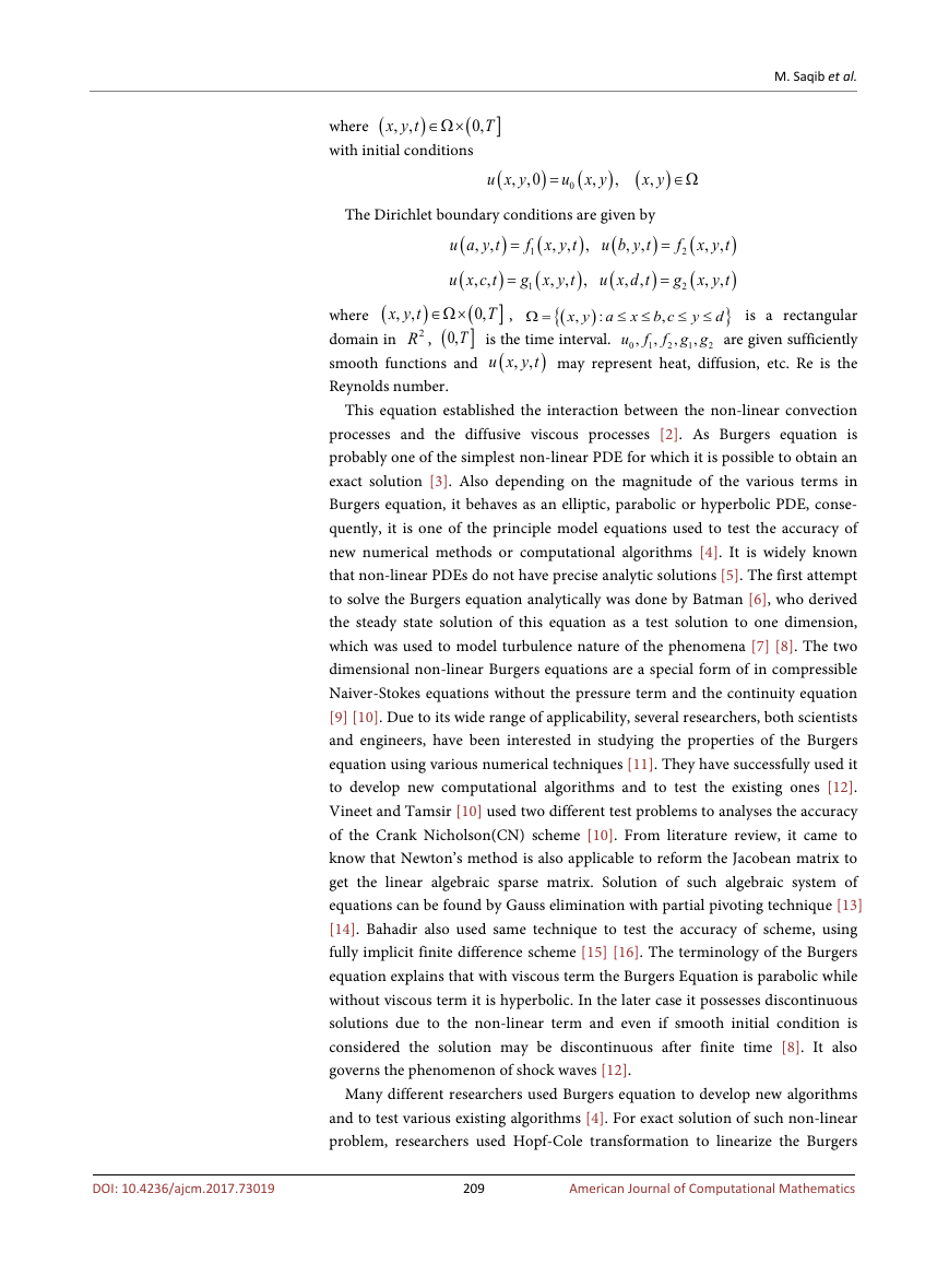
dimensional convection-diffusion equation is given by the following equation.
DOI: 10.4236/ajcm.2017.73019 Aug. 3, 2017
u
t
+
uu
x
+
uu
y
−
(
u
xx
+
u
yy
)
=
0
1
R
(1)
208
American Journal of Computational Mathematics
�
x y t
,
,
where (
(
0,
with initial conditions
∈Ω×
)
T
]
(
u x y
,
,0
)
=
u x y
,
0
(
)
,
(
x y
,
)
∈Ω
The Dirichlet boundary conditions are given by
)
(
u b y t
,
(
)
u x d t
,
f
1
g x y t
,
1
)
x y t
,
,
)
,
(
(
=
=
,
,
,
=
f
2
=
g
2
(
(
,
(
)
u a y t
,
)
(
u x c t
,
]
∈Ω×
T
,
,
{
(
)
(
where (
x y t
0,
,
,
]
2R , (
domain in
smooth functions and
Reynolds number.
)
,
a
:
0,T is the time interval.
Ω =
x y
,
≤ ≤
is a rectangular
x b c
,
≤ ≤
f g g are given sufficiently
u f
,
,
2
0
1
may represent heat, diffusion, etc. Re is the
y
,
(
u x y t
,
)
,
,
1
M. Saqib et al.
x y t
,
,
)
)
x y t
,
,
}
d
2
This equation established the interaction between the non-linear convection
processes and the diffusive viscous processes [2]. As Burgers equation is
probably one of the simplest non-linear PDE for which it is possible to obtain an
exact solution [3]. Also depending on the magnitude of the various terms in
Burgers equation, it behaves as an elliptic, parabolic or hyperbolic PDE, conse-
quently, it is one of the principle model equations used to test the accuracy of
new numerical methods or computational algorithms [4]. It is widely known
that non-linear PDEs do not have precise analytic solutions [5]. The first attempt
to solve the Burgers equation analytically was done by Batman [6], who derived
the steady state solution of this equation as a test solution to one dimension,
which was used to model turbulence nature of the phenomena [7] [8]. The two
dimensional non-linear Burgers equations are a special form of in compressible
Naiver-Stokes equations without the pressure term and the continuity equation
[9] [10]. Due to its wide range of applicability, several researchers, both scientists
and engineers, have been interested in studying the properties of the Burgers
equation using various numerical techniques [11]. They have successfully used it
to develop new computational algorithms and to test the existing ones [12].
Vineet and Tamsir [10] used two different test problems to analyses the accuracy
of the Crank Nicholson(CN) scheme [10]. From literature review, it came to
know that Newton’s method is also applicable to reform the Jacobean matrix to
get the linear algebraic sparse matrix. Solution of such algebraic system of
equations can be found by Gauss elimination with partial pivoting technique [13]
[14]. Bahadir also used same technique to test the accuracy of scheme, using
fully implicit finite difference scheme [15] [16]. The terminology of the Burgers
equation explains that with viscous term the Burgers Equation is parabolic while
without viscous term it is hyperbolic. In the later case it possesses discontinuous
solutions due to the non-linear term and even if smooth initial condition is
considered the solution may be discontinuous after finite time [8]. It also
governs the phenomenon of shock waves [12].
Many different researchers used Burgers equation to develop new algorithms
and to test various existing algorithms [4]. For exact solution of such non-linear
problem, researchers used Hopf-Cole transformation to linearize the Burgers
209
American Journal of Computational Mathematics
DOI: 10.4236/ajcm.2017.73019
�
M. Saqib et al.
equations into parabolic partial differential equation [17]. Some of the resear-
chers also tried to tackle the non-linear Burgers equation directly (without
Hopf-Cole transformation), by applying Crank-Nicholson finite difference
method to the linearized Burgers equation by Hopf-Cole transformation which
is unconditionally stable and is second order convergent, in both space and time
with no restriction on mesh size [10]. In another result due to Kutluay et al. a
direct approach via least square quadratic B-spline finite element method is
discussed [18]. Recently Pandey et al. discussed Douglas finite difference scheme
on linearized Burgers equation which is fourth order convergent in space and
second order convergent in time [1] [18].
1.1. Problem 1
From literature review, [19] we found that earlier work done by Mittal,Jain and
Holla in 2012 [20] on convection-diffusion equation in one dimension. We
extended our work to enhance our knowledge towards two dimensional Convection
diffusion equation.Two test problems were taken to understand the numerical
solution with finite difference schemes. By setting some parameters with arbitrary
constants in bounded domain
. Exact
x
solution of the above two dimensional equation is
y
+ −
2
0.5 tanh
(
u x y t
,
0.5, 0.5
}
0.5
: 0.5
−
,x y ∈Ω ,
where (
t > and R is a parameter, known as Reynolds number.
Boundary conditions and initial conditions can be taken from exact solution of
u(x,y,t) [21].
≤ ≤
≤ ≤
)
t R
(2)
Ω =
x y
,
{
(
(
x
−
,
)
=
−
y
)
0
)
1.2. Problem 2
In this problem the rectangular domain of two dimensional nonlinear convection-
)
diffusion Equation (1) is given as
. Exact
x y
1
,
solution of the above two dimensional equation is
≤ ≤
≤ ≤
Ω =
1,0
: 0
x
y
(
(
u x y t
,
,
)
=
(
x
1
+
1
y
+ −
2
)
t R
(3)
,
)
)
0
,x y ∈Ω ,
. where Ω is a rectangular domain in
where (
t > and R is a parameter, known as Reynolds number.
Boundary conditions and initial conditions can be taken from exact solution of
(
u x y t
2R . The main objective of the
,
(
),
u x t
paper is to find efficient solution of unknown
. Two test problems were
described to understand the numerical solution by taking two finite difference
schemes. Also Convection diffusion equation has been extensively studied to
describe various kinds of phenomena which can be seen from equation [21].
2. Numerical Methods
Numerical solution of the two dimensional non-linear equation in a finite
210
American Journal of Computational Mathematics
DOI: 10.4236/ajcm.2017.73019
�
M. Saqib et al.
)
(
)
(
=
−
=
hy
and
b a L
−
d c M
domain Ω . The first step is to choose integers L and M to define step sizes
hx
in x and y directions respectively.
xh and the interval [c, d]
Partition the interval [a, b] into L equal parts of width
yh . Place a grid by drawing vertical and horizontal
into M equal parts of width
lines through the points with coordinates (
for each
l
0,1,2,
=
also the lines
for each
x
x=
are grid lines, and their intersections are the mesh points of
l
the grid. For each mesh point in the interior of the grid, (
, for
l
=
, we apply different algorithms to
approximate the numerical solution to the problem in equation [21] also we
assume
where t is the time.
, where
0,1, 2,
)
x y
,l
m
m
=
and
L
−
=
−
c mk
and
and
a lh
nk n
,
x y
,l
= +
= +
lx
M
1,2,
L
y
0,1,
y=
1, 2,
NT
my
M
m
1
=
=
1
)
,
m
,
m
,
,
,
nt
2.1. Second Order Implicit Scheme
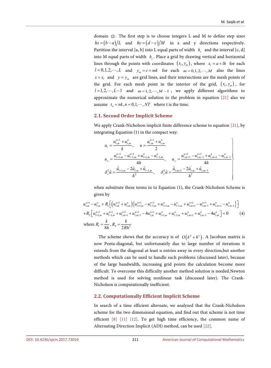
We apply Crank-Nicholson implicit finite difference scheme to equation [21], by
integrating Equation (1) in the compact way:
n
1
+
u
l m
,
n
u
l m
,
,
+
k
n
1
+
u
l m
,
u
=
n
1
+
u
l m
1,
+
−
n
1
+
u
l m
1,
−
n
u
l m
,
+
2
n
u
l m
1,
−
,
u
t
=
u
x
=
−
n
u
+
l m
1,
+
h
4
ˆ
u
2
+
l m
,
2
h
ˆ
u
l m
1,
−
ˆ
u
l m
1,
+
−
2
δ
x
ˆ
u
=
,
2
δ
y
ˆ
u
=
=
u
y
ˆ
u
l m
,
n
1
+
u
l m
,
1
+
−
n
1
+
u
l m
,
1
−
n
u
+
l m
,
h
4
ˆ
u
l m
1
,
−
−
1
+
+
ˆ
u
2
l m
,
2
h
−
n
u
l m
,
1
−
1
+
+
n
u
l m
,
when substitute these terms in to Equation (1), the Crank-Nicholson Scheme is
given by
(
R u
1
n
1
+
u
l m
1,
−
k
h
8
){
n
1
+
u
l m
1,
+
n
1
+
u
+
l m
,
1
−
n
1
+
u
l m
1
,
+
k
Rh
n
u
l m
,
n
u
4
l m
,
n
u
l m
,
0
n
1
+
u
4
l m
,
n
1
+
u
l m
,
1
+
n
1
+
u
l m
,
1
−
n
u
l m
1,
+
n
u
l m
1,
+
n
u
l m
1,
−
n
1
+
u
l m
1,
−
n
u
l m
1,
−
n
1
+
l m
1,
+
(4)
n
u
l m
,
n
u
l m
,
n
u
l m
,
1
+
n
1
+
l m
,
R
2
R
1
}
+
−
+
−
+
−
+
−
+
+
−
+
+
+
+
−
=
=
=
2
1
+
1
−
1
−
,
2
−
n
1
+
u
l m
,
R u
2
+
where
(
O k
)
2
2
h+
The scheme shows that the accuracy is of
. A Jacobian matrix is
now Penta-diagonal, but unfortunately due to large number of iterations it
extends from the diagonal at least n entries away in every direction,but another
methods which can be used to handle such problems (discussed later), because
of the large bandwidth, increasing grid points the calculation become more
difficult. To overcome this difficulty another method solution is needed.Newton
method is used for solving nonlinear task (discussed later). The Crank-
Nicholson is computationally inefficient.
2.2. Computationally Efficient Implicit Scheme
In search of a time efficient alternate, we analyzed that the Crank-Nicholson
scheme for the two dimensional equation, and find out that scheme is not time
efficient [8] [11] [12]. To get high time efficiency, the common name of
Alternating Direction Implicit (ADI) method, can be used [22].
211
American Journal of Computational Mathematics
DOI: 10.4236/ajcm.2017.73019
�
M. Saqib et al.
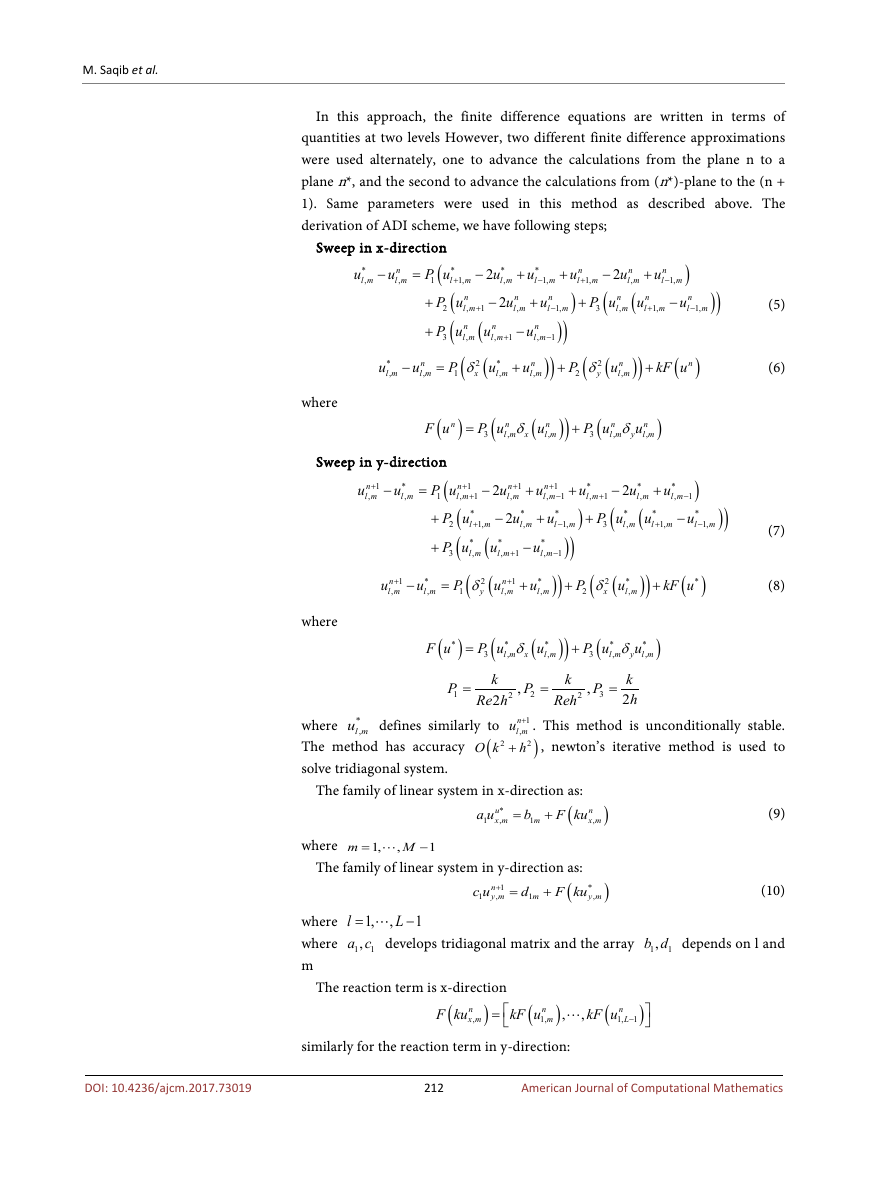
In this approach, the finite difference equations are written in terms of
quantities at two levels However, two different finite difference approximations
were used alternately, one to advance the calculations from the plane n to a
plane n*, and the second to advance the calculations from (n*)-plane to the (n +
1). Same parameters were used in this method as described above. The
derivation of ADI scheme, we have following steps;
=
−
*
u
l m
,
n
u
l m
,
Sweep in x-direction
(
*
P u
l m
1,
1
+
(
n
P u
+
l m
,
2
(
P u
3
(
2
P
δ
x
1
n
u
l m
,
*
u
l m
,
n
l m
,
+
−
=
−
*
u
2
+
l m
,
n
u
2
−
l m
,
−
1
+
(
1
+
n
u
l m
,
(
*
u
l m
,
+
*
u
l m
1,
−
n
u
+
l m
1,
−
n
u
l m
,
1
−
+
n
u
l m
,
)
)
)
)
+
n
n
u
u
2
−
+
l m
l m
,
1,
+
(
)
n
n
u
P u
+
l m
l m
1,
3
,
+
(
)
n
u
l m
1,
−
n
u
−
l m
1,
−
)
)
(5)
(
2
δ
y
(
P
2
n
u
l m
,
)
)
+
(
kF u
n
)
(6)
where
n
)
=
−
*
u
l m
,
(
P u
3
n
1
+
u
l m
,
(
F u
Sweep in y-direction
(
n
1
+
P u
l m
1
,
1
+
(
*
P u
+
l m
1,
2
+
(
(
*
*
P u
u
l m
l m
,
3
,
(
(
2
P
δ
y
1
n
1
+
u
l m
,
*
u
l m
,
=
−
+
−
=
where
*
)
=
(
F u
(
P u
3
k
Re h
2
defines similarly to
(
2
O k
P
1
=
*
,l mu
where
The method has accuracy
solve tridiagonal system.
)
)
+
+
)
)
k
Reh
n
δ
l m x
,
(
n
u
l m
,
)
)
+
(
P u
3
n
δ
l m y
,
n
u
l m
,
)
+
n
1
+
u
2
l m
,
*
u
2
−
l m
,
−
1
+
+
n
1
+
u
l m
,
1
−
*
u
+
l m
1,
−
*
u
l m
,
1
−
*
u
l m
,
)
+
*
u
2
−
+
l m
1
,
+
(
*
*
u
P u
l m
l m
1,
3
,
+
*
u
l m
,
1
−
*
u
−
l m
1,
−
(
)
)
)
(7)
n
1
+
u
l m
,
+
*
u
l m
,
)
)
(
2
δ
x
(
P
2
*
u
l m
,
)
)
+
(
kF u
*
)
(8)
*
δ
l m x
,
(
*
u
l m
,
(
P u
3
*
u
l m
,
)
,
P
2
=
2
,
P
3
2
*
δ
l m y
,
k
h
2
=
1
n
l mu + . This method is unconditionally stable.
,
, newton’s iterative method is used to
h+
2
)
The family of linear system in x-direction as:
(
n
F ku
x m
,
a u
1
b
m
1
u
*
x m
,
=
+
where
m
=
1,
−
M
,
1
The family of linear system in y-direction as:
(
*
F ku
y m
,
n
1
+ =
y m
,
d
m
1
c u
1
+
)
)
,
1
1,
L
−
l
=
1,a c develops tridiagonal matrix and the array
1
where
where
m
The reaction term is x-direction
=
)
similarly for the reaction term in y-direction:
(
n
kF u
1,
(
F ku
n
x m
,
)
m
,
kF u −
L
1
n
1,
(
,
(9)
(10)
,b d depends on l and
1
1
)
DOI: 10.4236/ajcm.2017.73019
212
American Journal of Computational Mathematics
�
M. Saqib et al.
(
F ku
*
y l
,
)
(
*
kF u
1,
=
M
1
−
)
,
,
(
*
kF u
1,1
)
finally the scheme makes tridiagonal family of linear system.Iterative methods
was carried out to solved this system. The trick used in constructing the ADI
scheme is to split time step into two, and apply two different stencils in each half
time step, therefore to increment time by one time step in grid point, we first
compute both of these stencils are chosen such that the resulting linear system is
tridiagonal [5] [7] [8] [9] [11] [17] [22]. To obtain the numerical solution, we
need to solve a non-linear tridiagonal system at each time step. We have done
this by using Newton’s iterative method
Algorithm 1
To construct Newton iterative method for the two dimensional Convection-
diffusion equation. The non-linear system in equations [23] and [24], can be
written in the form:
) 0
(
G S =
(11)
where
S
≈
n
1
+
u
=
S
1,
m
,
S
2,
m
,
,
S
(
2
L
−
)
2 ,
m
n
1
+
u
m
1,
,
u
n
1
+
m
2,
,
n
1
+
u
m
3,
,
,
u
n
1
+
L m
1,
−
T
T
1
+
n
mu
:
G −
(
L
2
=
T
=
,
,
,
m
m
G
G G
1,
2,
were system of
nonlinear equations obtained from the system in [23] and [24]. The system of
equations, is solved by Newton’s iterative method using the following steps
, where
G G
1,
2,
G −
(
L
)
2 ,
)
2 ,
m
m
m
m
,
,
,
2
1) Specify
k =
2) For
( )0u
0,1,2,
as an initial approximation.
until convergence achieve.
)
(
)
R u
= −
u
∆
)
k
k
k
(
)
(
)
(
(
A u
(
k
)
)
(
,
u
)k
(
)
• Solve the linear system
)
(
k
1k
+ =
u
u
• Specify
+ ∆
(
)
is (
m m×
A u
where
Jacobian matrix, which is computed analytically and
)ku∆
(
is the correction vector. In the iteration method solution at the previous
time step is taken as the initial guess. Iteration at each time step is stopped when
(
)k
R u
with Tol is a very small prescribed value. The linear system
obtained from Newton’s iterative method, is solved by Court’s method.
Convergence done with iterations along less CPU time [5] [14].
Tol
≤
∞
(
)
Algorithm 2
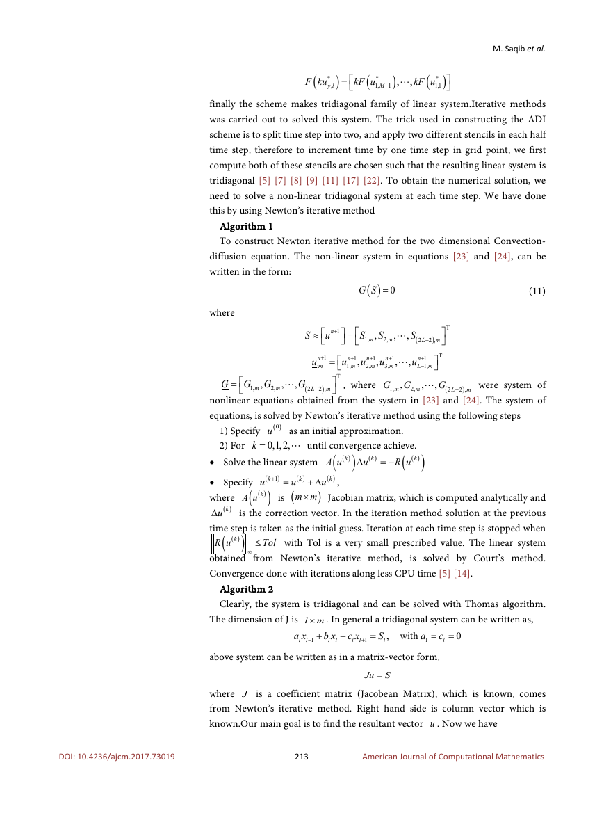
Clearly, the system is tridiagonal and can be solved with Thomas algorithm.
The dimension of J is l m× . In general a tridiagonal system can be written as,
c
l
above system can be written as in a matrix-vector form,
, with
a x
l
l
b x
l
l
c x
l
l
a
1
+
+
=
=
S
1
+
1
−
l
=
0
Ju
S=
where J is a coefficient matrix (Jacobean Matrix), which is known, comes
from Newton’s iterative method. Right hand side is column vector which is
known.Our main goal is to find the resultant vector u . Now we have
213
American Journal of Computational Mathematics
DOI: 10.4236/ajcm.2017.73019
�
M. Saqib et al.
J
0
0
0
0
0
c
2
c
1
b
2
b
0
1
a
0
2
=
a
n
1
−
c
n
1
−
b
n
1
−
b
n
a
n
]
]
n
t
u
s
n
t
u
=
S
=
2
,
[
u u u
,
1
3
[
s s
,
1
2
s
3
,
,
,
,
,
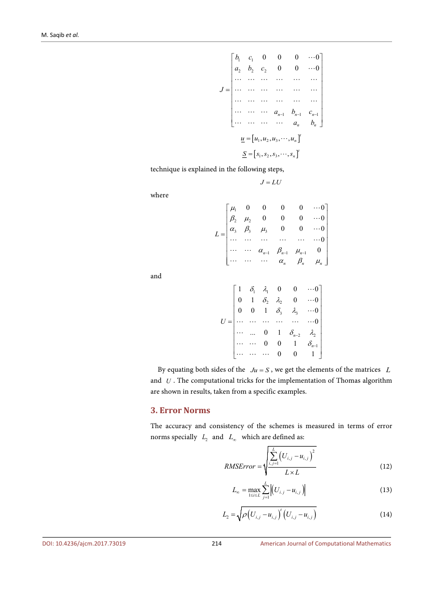
technique is explained in the following steps,
LU=
J
where
and
L
2
0
0
0
0
0
0
0
0
0
µ
1
0
0
β µ
2
0
α β µ
3
3
=
0
0
n
n
1
−
α β µ
n
α β µ
n
1
−
1
−
n
n
3
U
δ λ
1
1
1
0
0
δ λ
2
2
1
0
0
δ λ
3
0
1
0
0
0
0
=
0
...
0
λ
2
0
δ
n
1
−
1
δ
n
−
1
0
1
0
0
3
2
By equating both sides of the Ju
S= , we get the elements of the matrices L
and U . The computational tricks for the implementation of Thomas algorithm
are shown in results, taken from a specific examples.
3. Error Norms
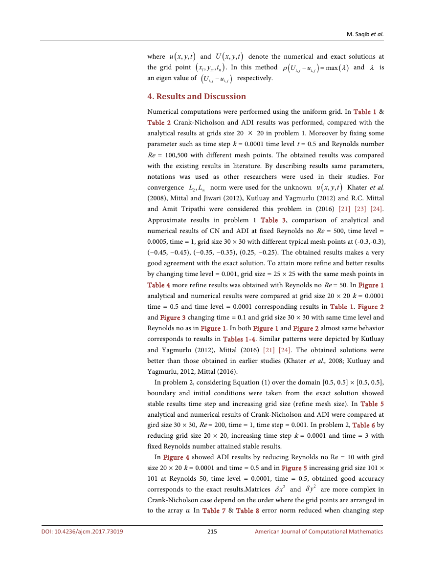
The accuracy and consistency of the schemes is measured in terms of error
norms specially
2L and L∞ which are defined as:
)2
(
U
∑
u
i
−
L
i
j
j
,
,
RMSError
=
i
,
j
1
=
L L
×
(
U
i j
.
−
u
i
,
j
)
L
∞
=
L
∑
max
i L j
1
≤ ≤
1
=
(12)
(13)
DOI: 10.4236/ajcm.2017.73019
(
U
ρ=
i j
,
L
2
−
u
i j
,
t
) (
U
i j
,
−
u
i j
,
)
(14)
214
American Journal of Computational Mathematics
�
M. Saqib et al.
,
)
)
(
)
λ
i j
,
i j
,
−
u
i j
,
i j
,
=
max
(
U
ρ
2,L L∞ norm were used for the unknown
,
. In this method
)
respectively.
denote the numerical and exact solutions at
and λ is
)
(
(
U x y t
u x y t
,
,
where
and
the grid point (
)
x y t
,
,
m n
l
an eigen value of (
u−
U
4. Results and Discussion
Numerical computations were performed using the uniform grid. In Table 1 &
Table 2 Crank-Nicholson and ADI results was performed, compared with the
analytical results at grids size 20 × 20 in problem 1. Moreover by fixing some
parameter such as time step k = 0.0001 time level t = 0.5 and Reynolds number
Re = 100,500 with different mesh points. The obtained results was compared
with the existing results in literature. By describing results same parameters,
notations was used as other researchers were used in their studies. For
convergence
Khater et al.
(2008), Mittal and Jiwari (2012), Kutluay and Yagmurlu (2012) and R.C. Mittal
and Amit Tripathi were considered this problem in (2016) [21] [23] [24].
Approximate results in problem 1 Table 3, comparison of analytical and
numerical results of CN and ADI at fixed Reynolds no Re = 500, time level =
0.0005, time = 1, grid size 30 × 30 with different typical mesh points at (-0.3,-0.3),
(−0.45, −0.45), (−0.35, −0.35), (0.25, −0.25). The obtained results makes a very
good agreement with the exact solution. To attain more refine and better results
by changing time level = 0.001, grid size = 25 × 25 with the same mesh points in
Table 4 more refine results was obtained with Reynolds no Re = 50. In Figure 1
analytical and numerical results were compared at grid size 20 × 20 k = 0.0001
time = 0.5 and time level = 0.0001 corresponding results in Table 1. Figure 2
and Figure 3 changing time = 0.1 and grid size 30 × 30 with same time level and
Reynolds no as in Figure 1. In both Figure 1 and Figure 2 almost same behavior
corresponds to results in Tables 1-4. Similar patterns were depicted by Kutluay
and Yagmurlu (2012), Mittal (2016) [21] [24]. The obtained solutions were
better than those obtained in earlier studies (Khater et al., 2008; Kutluay and
Yagmurlu, 2012, Mittal (2016).
(
u x y t
,
,
)
In problem 2, considering Equation (1) over the domain [0.5, 0.5] × [0.5, 0.5],
boundary and initial conditions were taken from the exact solution showed
stable results time step and increasing grid size (refine mesh size). In Table 5
analytical and numerical results of Crank-Nicholson and ADI were compared at
gird size 30 × 30, Re = 200, time = 1, time step = 0.001. In problem 2, Table 6 by
reducing grid size 20 × 20, increasing time step k = 0.0001 and time = 3 with
fixed Reynolds number attained stable results.
In Figure 4 showed ADI results by reducing Reynolds no Re = 10 with gird
size 20 × 20 k = 0.0001 and time = 0.5 and in Figure 5 increasing grid size 101 ×
101 at Reynolds 50, time level = 0.0001, time = 0.5, obtained good accuracy
2yδ are more complex in
corresponds to the exact results.Matrices
Crank-Nicholson case depend on the order where the grid points are arranged in
to the array u. In Table 7 & Table 8 error norm reduced when changing step
2xδ and
215
American Journal of Computational Mathematics
DOI: 10.4236/ajcm.2017.73019
�



 2023年江西萍乡中考道德与法治真题及答案.doc
 2012年重庆南川中考生物真题及答案.doc
 2013年江西师范大学地理学综合及文艺理论基础考研真题.doc
 2020年四川甘孜小升初语文真题及答案I卷.doc
 2020年注册岩土工程师专业基础考试真题及答案.doc
 2023-2024学年福建省厦门市九年级上学期数学月考试题及答案.doc
 2021-2022学年辽宁省沈阳市大东区九年级上学期语文期末试题及答案.doc
 2022-2023学年北京东城区初三第一学期物理期末试卷及答案.doc
 2018上半年江西教师资格初中地理学科知识与教学能力真题及答案.doc
 2012年河北国家公务员申论考试真题及答案-省级.doc
 2020-2021学年江苏省扬州市江都区邵樊片九年级上学期数学第一次质量检测试题及答案.doc
 2022下半年黑龙江教师资格证中学综合素质真题及答案.doc