SCAPE: Shape Completion and Animation of People
Dragomir Anguelov∗
Praveen Srinivasan∗
Daphne Koller∗
StanfordUniversity
Sebastian Thrun∗
Jim Rodgers∗
James Davis†
University of California, Santa Cruz
Figure 1: Animation of a motion capture sequence taken for a subject, of whom we have a single body scan. The muscle deformations are synthesized
automatically from the space of pose and body shape deformations.
Abstract
We introduce the SCAPE method (Shape Completion and Anima-
tion for PEople) — a data-driven method for building a human shape
model that spans variation in both subject shape and pose. The
method is based on a representation that incorporates both artic-
ulated and non-rigid deformations. We learn a pose deformation
model that derives the non-rigid surface deformation as a function
of the pose of the articulated skeleton. We also learn a separate
model of variation based on body shape. Our two models can be
combined to produce 3D surface models with realistic muscle defor-
mation for different people in different poses, when neither appear
in the training set. We show how the model can be used for shape
completion — generating a complete surface mesh given a limited
set of markers specifying the target shape. We present applications
of shape completion to partial view completion and motion capture
animation. In particular, our method is capable of constructing a
high-quality animated surface model of a moving person, with real-
istic muscle deformation, using just a single static scan and a marker
motion capture sequence of the person.
CR Categories: I.3.5 [Computer Graphics]: Computational Ge-
ometry and Object Modeling—Hierarchy and geometric transfor-
mations; I.3.7 [Computer Graphics]: Three-Dimensional Graphics
and Realism—Animation
Keywords: synthetic actors, deformations, animation, morphing
1
Graphics applications often require a complete surface model for
rendering and animation. Obtaining a complete model of a partic-
ular person is often difficult or impossible. Even when the person
Introduction
∗e-mail: {drago,praveens,koller,thrun,jimkr}@cs.stanford.edu
†e-mail: davis@cs.ucsc.edu
Copyright © 2005 by the Association for Computing Machinery, Inc.
Permission to make digital or hard copies of part or all of this work for personal or classroom
use is granted without fee provided that copies are not made or distributed for commercial
advantage and that copies bear this notice and the full citation on the first page. Copyrights
for components of this work owned by others than ACM must be honored. Abstracting with
credit is permitted. To copy otherwise, to republish, to post on servers, or to redistribute to
lists, requires prior specific permission and/or a fee. Request permissions from Permissions
Dept, ACM Inc., fax +1 (212) 869-0481 or e-mail permissions@acm.org.
© 2005 ACM 0730-0301/05/0700- 0408 $5.00
408
can be constrained to remain motionless inside of a Cyberware full
body scanner, incomplete surface data is obtained due to occlusions.
When the task is to obtain a 3D sequence of the person in motion,
the situation can be even more difficult. Existing marker-based mo-
tion capture systems usually provide only sparse measurements at a
small number of points on the surface. The desire is to map such
sparse data into a fully animated 3D surface model.
This paper introduces the SCAPE method (Shape Completion
and Animation for PEople) — a data-driven method for building
a unified model of human shape. Our method learns separate mod-
els of body deformation — one accounting for changes in pose and
one accounting for differences in body shape between humans. The
models provide a level of detail sufficient to produce dense full-
body meshes, and capture details such as muscle deformations of
the body in different poses. Importantly, our representation of de-
formation allows the pose and the body shape deformation spaces to
be combined in a manner which allows proper deformation scaling.
For example, our model can correctly transfer the deformations of a
large person onto a small person and vice versa.
The pose deformation component of our model is acquired from a
set of dense 3D scans of a single person in multiple poses. A key as-
pect of our pose model is that it decouples deformation into a rigid
and a non-rigid component. The rigid component of deformation
is described in terms of a low degree-of-freedom rigid body skele-
ton. The non-rigid component captures the remaining deformation
such as flexing of the muscles. In our model, the deformation for
a body part is dependent only on the adjacent joints. Therefore, it
is relatively low dimensional, allowing the shape deformation to be
learned automatically, from limited training data.
Our representation also models shape variation that occurs across
different individuals. This model component can be acquired from
a set of 3D scans of different people in different poses. The
shape variation is represented by using principal component anal-
ysis (PCA), which induces a low-dimensional subspace of body
shape deformations. Importantly, the model of shape variation does
not get confounded by deformations due to pose, as those are ac-
counted for separately. The two parts of the model form a single
unified framework for shape variability of people. The framework
can be used to generate a complete surface mesh given only a suc-
cinct specification of the desired shape — the angles of the human
skeleton and the eigen-coefficients describing the body shape.
We apply our model to two important graphics tasks. The first is
partial view completion. Most scanned surface models of humans
�
have significant missing regions. Given a partial mesh of a person
for whom we have no previous data, our method finds the shape that
best fits the observed partial data in the space of human shapes. The
model can then be used to predict a full 3D mesh. Importantly, be-
cause our model also accounts for non-rigid pose variability, muscle
deformations associated with the particular pose are predicted well
even for unobserved parts of thebody.
The second task is producing a full 3D animation of a moving
person from marker motion capture data. We approach this problem
as a shape completion task. The input to our algorithm is a single
scan of the person and a time series of extremely sparse data — the
locations of a limited set of markers (usually between 50 and 60)
placed on the body. For each frame in the sequence, we predict the
full 3D shape of the person, in a pose consistent with the observed
marker positions. Applying this technique to sequences of motion
capture data produces full-body human 3D animations. We show
that our method is capable of constructing high-quality animations,
with realistic muscle deformation, for people of whom we have a
single range scan.
In both of these tasks, our method allows for variation of the in-
dividual body shape. For example, it allows for the synthesis of a
person with a different body shape, not present in the original set of
scans. The motion for this new character can also be synthesized,
either based on a motion capture trajectory for a real person (of sim-
ilar size), or keyframed by an animator. Thus, our approach makes
it possible to create realistic shape completions and dense 3D ani-
mations for people whose exact body shape is not included in any
of the available datasources.
2 Related Work
The recent example-based approaches for learning deformable hu-
man models represent deformation by point displacements of the
example surfaces, relative to a generic template shape. For model-
ing pose deformation, the template shape is usually assumed to be
an articulated model. A popular animation approach called skin-
ning (described in [Lewis et al. 2000]) assumes that the point dis-
placements are generated by a weighted set of (usually linear) in-
fluences from neighboring joints. A more sophisticated method was
presented by Allen et al. [2002], who register an articulated model
(represented as a posable subdivision template) to scans of a human
in different poses. The displacements for a new pose are predicted
by interpolating from a set of example scans with similar joint an-
gles. A variety of related methods [Lewis et al. 2000; Sloan et al.
2001; Wang and Phillips 2002; Mohr and Gleicher 2003] differ only
in the details of representing the point displacements, and in the par-
ticular interpolation method used. Models of pose deformation are
learned not only from 3D scans, but also by combining shape-from-
silhouette and marker motion capture sequences [Sand et al.2003].
However, none of the above approaches learn a model of the shape
changes between different individuals.
To model body shape variation across different people, Allen et
al. [2003] morph a generic template shape into 250 scans of differ-
ent humans in the same pose. The variability of human shape is
captured by performing principal component analysis (PCA) over
the displacements of the template points. The model is used for
hole-filling of scans and fitting a set of sparse markers for people
captured in the standard pose. Another approach, by Seo and Thal-
mann [2003], decomposes the body shape deformation into a rigid
and a non-rigid component, of which the latter is also represented as
a PCA over point displacements. Neither approach learns a model of
pose deformation. However, they demonstrate preliminary anima-
tion results by using expert-designed skinning models. Animation is
done by bringing the space of body shapes and the skinning model
into correspondence (this can be done in a manual or semi-automatic
way [Hilton et al. 2002]), and adding the point displacements ac-
counting for pose deformation to the human shape. Such skinning
models are part of standard animation packages, but since they are
usually not learned from scan data, they usually don’t model muscle
deformation accurately.
Figure 2: The mesh processing pipeline used to generate our training set.
(a) We acquired two data sets spanning the shape variability due to differ-
ent human poses and different physiques. (b) We select a few markers by
hand mapping the template mesh and each of the range scans. (c) We apply
the Correlated Correspondence algorithm, which computes numerous addi-
tional markers. (d) We use the markers as input to a non-rigid registration
algorithm, producing fully registered meshes. (e) We apply a skeleton re-
construction algorithm to recover an articulated skeleton from the registered
meshes. (f) We learn the space of deformations due to pose andphysique.
An obvious approach for building a data-driven model of pose
and body shape deformation would be to integrate two existing
methods in a similar way. The main challenge lies in finding a good
way to combine two distinct deformation models based on point
displacements. Point displacements cannot be multiplied in a mean-
ingful way; adding them ignores an important notion of scale. For
example, pose displacements learned on a large individual cannot
be added to the shape of a small individual without undesirable ar-
tifacts. This problem has long been known in the fields of deforma-
tion transfer and expression cloning [Noh and Neumann 2001]. In
order to address it, we take an inspiration in the deformation transfer
method of Sumner and Popovic´ [2004]. It shows how to retarget the
deformation of one mesh to another, assuming point-to-point cor-
respondences between them are available. The transfer maintains
proper scaling of deformation, by representing the deformation of
each polygon using a 3 × 3 matrix. It suggests a way of mapping
pose deformations onto a variety of human physiques. However, it
does not address the task of representing and learning a deformable
human model, which is tackled in thispaper.
Multilinear models, which are closely related to our work, have
been applied for modeling face variation in images [Vasilescu and
Terzopoulos 2002]. A generative model of human faces has to ad-
dress multiple factors of image creation such as illumination, ex-
pression and viewpoint. The face is modeled as a product of linear
appearance models, corresponding to influences of the various fac-
tors. Ongoing work is applying multilinear approaches to model 3D
face deformation [Vlasic et al. 2004]. Our method adapts the idea to
the space of human body shapes, which exhibits articulated structure
that makes human body modeling different from face modeling. In
particular, we directly relate surface deformations to the underlying
body skeleton. Such a model would not be sufficient to address face
deformation, because a significant part of the deformation is purely
muscle-based, and is not correlated with the skeleton.
Our shape-completion application is related to work in the area
of hole-filling. Surfaces acquired with scanners are typically incom-
plete and contain holes. A common way to complete these holes is
to fill them with a smooth surface patch that meets the boundary
conditions of the hole [Curless and Levoy 1996; Davis et al. 2002;
Liepa 2003]. These approaches work well when the holes are small
compared to the geometric variation of the surface. Our application,
409
�
by contrast, requires the filling of huge holes (e.g., in some experi-
ments more than half of the surface was not observed; in others we
are only provided with sparse motion capture data) and we address
it with a model-based method. Other model-based solutions for hole
filling were proposed in the past. Ka¨hler et al. [2002] and Szeliski
and Lavalle´e [1996] use volumetric template-based methods for this
problem. These approaches work well for largely convex objects,
such as a human head, but are not easily applied to objects with
branching parts, such as the human body. While the work of Allen
et al. [2003] can be used for hole-filling of human bodies, it can
only do so if the humans are captured in a particular pose.
Marker motion capture systems are widely available, and can
be used for obtaining high-quality 3D models of a moving per-
son. Existing animation methods (e.g. [Allen et al. 2002; Seo and
Magnenat-Thalmann 2003]) do not utilize the marker data and as-
sume the system directly outputs the appropriate skeleton angles.
They also do not handle body shape variation well, as previously
discussed. Both of these limitations are lifted in ourwork.
3 Acquiring and Processing Data Meshes
The SCAPE model acquisition is data driven, and all the information
about the shape is derived from a set of range scans. This section
describes the basic pipeline for data acquisition andpre-processing
of the data meshes. This pipeline, displayed in in Fig. 2, consists
largely of a combination of previously published methods. The spe-
cific design of the pipeline is inessential for the main contribution
of this paper; we describe it first to introduce the type of data used
for learning our model.
Range Scanning We acquired our surface data using a Cyber-
ware WBX whole-body scanner. The scanner captures range scans
from four directions simultaneously and the models contain about
200K points. We used this scanner to construct full-body instance
meshes by merging the four scan views [Curless and Levoy 1996]
and subsampling the instances to about 50,000 triangles [Garland
and Heckbert 1997].
Using the process above, we obtained two data sets: a pose data
set, which contains scans of 70 poses of a particular person in a
wide variety of poses, and a body shape data set, which contains
scans of 37 different people in a similar (but not identical) pose. We
also added eight publicly available models from the CAESAR data
set [Allen et al. 2003] to our data set of individuals.
We selected one of the meshes in the pose data set to be thetem-
plate mesh; all other meshes will be called instance meshes. The
function of the template mesh is to serve as a point of reference
for all other scans. The template mesh is hole-filled using an al-
gorithm by Davis et al.[2002]. In acquiring the template mesh, we
ensured that only minor holes remained mostly between the legs and
the armpits. The template mesh and some sample instance meshes
are displayed in Fig. 2(a). Note that the head region is smoothed in
some of the figures, in order to hide the identity of the scan subjects;
the complete scans were used in the learning algorithm.
Correspondence The next step in the data acquisition pipeline
brings the template mesh into correspondence with each of the other
mesh instances. Current non-rigid registration algorithms require
that a set of corresponding markers between each instance mesh
and the template is available (the work of Allen et al. [2003] uses
about 70 markers for registration). We obtain the markers using an
algorithm called Correlated Correspondence (CC) [Anguelov et al.
2005]. The CC algorithm computes the consistent embedding of
each instance mesh into the template mesh, which minimizes defor-
mation, and matches similar-looking surface regions. To break the
scan symmetries, we initialize the CC algorithm by placing 4–10
markers by hand on each pair of scans. The result of the algorithm
is a set of 140–200 (approximate) correspondence markers between
the two surfaces, as illustrated in Fig.2(c).
Non-rigid Registration Given a set of markers between two
meshes, the task of non-rigid registration is well understood
and
a variety of algorithms exist [Allen et al. 2002; Ha¨hnel et al. 2003;
Sumner and Popovic´ 2004]. The task is to bring the meshes
into
410
close alignment, while simultaneously aligning the markers. We ap-
ply a standard algorithm [Ha¨hnel et al. 2003] to register the template
mesh with all of the meshes in our data set. As a result, we obtain
a set of meshes with the same topology, whose shape approximates
well the surface in the original Cyberware scans. Several of the re-
sulting meshes are displayed in Fig. 2(d).
Recovering the Articulated Skeleton As discussed in the intro-
duction, our model uses a low degree-of-freedom skeleton to model
the articulated motion. We construct a skeleton for our template
mesh automatically, using only the meshes in our data set. We ap-
plied the algorithm of [Anguelov et al. 2004], which uses a set of
registered scans of a single subject in a variety of configurations.
The algorithm exploits the fact that vertices on the same skeleton
joint are spatially contiguous, and exhibit similar motion across the
different scans. It automatically recovers a decomposition of the
object into approximately rigid parts, the location of the parts in the
different object instances, and the articulated object skeleton linking
the parts. Based on our pose data set, the algorithm automatically
constructed a skeleton with 18 parts. The algorithm broke both the
crotch area and the chest area into two symmetric parts, resulting in
a skeleton which was not tree-structured. To facilitate pose editing,
we combined the two parts in each of these regions into one. The
result was a tree-structured articulated skeleton with 16 parts.
Data Format and Assumptions The resulting data set con-
sists of a model mesh X and a set of instance meshes Y =
{Y1,...,YN }. The model mesh X = {VX,PX} has a set of vertices
VX = {x1,..., xM} and a set of triangles PX= {p1,..., pP}. The in-
stance meshes are of two types: scans of the same person in various
poses, and scans of multiple people in approximately the same pose.
As a result of our pre-processing, we can assume that each in-
stance mesh has the same set of points and triangles as the model
mesh, albeit in different configurations. Thus, let Y i = {yi ,...,yi }
M
be the set of points in instance mesh Y i. As we also mapped each of
the instance meshes onto our articulated model in the pre-processing
phase, we also have, for each mesh Y i, a set of absolute rotations Ri
for the rigid parts of the model, where Ri is the rotation of joint f in
instance i.
The data acquisition and pre-processing pipeline provides us with
exactly this type of data; however, any other technique for generat-
ing similar data will also be applicable to our learning and shape
completionapproach.
f
1
4 Pose Deformation
This and the following sections describe the SCAPE model, which is
the main contribution of this paper. In the SCAPE model,deforma-
tions due to changes in pose and body shape are modeled separately.
In this section, we focus on learning the pose deformation model.
4.1 Deformation Process
We want to model the deformations which align the template with
each mesh Y i in the data set containing different poses of ahuman.
The deformations are modeled for each triangle pk of the template.
We use a two-step, translation invariant representation of triangle
deformations, accounting for a non-rigid and a rigid component of
the deformation. Let triangle pk contain the points xk,1, xk,2, xk,3.
We apply our deformations in terms of the triangle’s local coor-
dinate system, obtained by translating point xk,1 to the global ori-
gin. Thus, the deformations will be applied to the triangle edges
vˆk,j = xk, j −xk,1, j = 2,3.
First, we apply a 3 × 3 linear transformation matrix Qi to the tri-
angle. This matrix, which corresponds to a non-rigid pose-induced
deformation, is specific to each triangle pk and each pose Yi. The
deformed polygon is then rotated by Ri , the rotation of its rigid part
in the articulated skeleton. The same rotation is applied to all trian-
gles that belong to that part. Letting f[k] be the body part associated
f
k
�
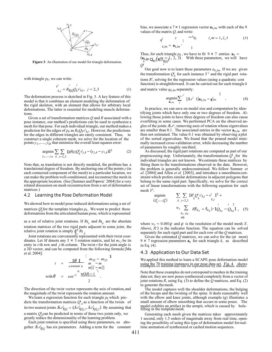
Figure 3: An illustration of our model for triangle deformation.
with triangle pk, we can write:
i
vi
k, j = Rf[k]Qkvˆk,j,
i
j = 2,3
(1)
The deformation process is sketched in Fig. 3. A key feature of this
model is that it combines an element modeling the deformation of
the rigid skeleton, with an element that allows for arbitrary local
deformations. The latter is essential for modeling muscle deforma-
tions.
Given a set of transformation matrices Q and R associated with a
pose instance, our method’s predictions can be used to synthesize a
mesh for that pose. For each individual triangle, our method makes a
prediction for the edges of pk as RkQkvˆk,j. However, the predictions
for the edges in different triangles are rarely consistent. Thus,
to
construct a single coherent mesh, we solve for the location of the
points y1,..., yM that minimize the overall least squares error:
argmin if[k]Qi vˆj,k −(y j,k − y1,k)I2
y1 ,...,yM k j=2,3
IR
k
(2)
Learning the Pose Deformation Model
Note that, as translation is not directly modeled, the problem has a
translational degree of freedom. By anchoring one of the points y (in
each connected component of the mesh) to a particular location, we
can make the problem well-conditioned, and reconstruct the mesh in
the appropriate location. (See [Sumner and Popovic´ 2004] for a very
related discussion on mesh reconstruction from a set of deformation
matrices.)
4.2
We showed how to model pose-induced deformations using a set of
matrices Qi for the template triangles pk . We want to predict these
deformations from the articulated human pose, which is represented
as a set of relative joint rotations. If Rf1 and Rf2 are the absolute
rotation matrices of the two rigid parts adjacent to some joint, the
relative joint rotation is simply RT Rf .
2
Joint rotations are conveniently represented with their twist coor-
dinates. Let M denote any 3 × 3 rotation matrix, and let mi j be its
entry in i-th row and j-th column. The twist t for the joint angle is
a 3D vector, and can be computed from the following formula [Ma
et al. 2004]:
f1
k
t =
withθ = cos−1
l
「
Iθ I
2sinIθ I
a
m32 − m23
m − m
13
31
m21 − m12
\
tr(M)−1
.
2
The direction of the twist vector represents the axis of rotation,and
the magnitude of the twist represents the rotation amount.
We learn a regression function for each triangle pk which pre-
dicts the transformation matrices Qi as a function of the twists of
i
its two nearest joints .6.ri
f[k],2). By assuming that
a matrix Qi can be predicted in terms of these two joints only, we
greatly reduce the dimensionality of the learning problem.
Each joint rotation is specified using three parameters, so alto-
constant
has six parameters. Adding a term for the
= (.6.r
k
i
f[k],1
gether .6.ri
,.6.r
f[k]
k
f[k]
bias, we associate a 7×1 regression vector ak,lm with each of the 9
values of the matrix Q, and write:
.6.rf[k
i
l,m = 1,2,3
「
(3)
1
T
qi
k,lm = ak,lm·
]
1
i
l, m = 1, 2, 3). With these parameters, we will have
Thus, for each triangle pk , we have to fit 9 × 7 entries ak =
(ak,lm :
k = Qak(.6.rf[k]).
Qi
Our goal now is to learn these parameters ak,lm. If we are given
the transformation Qi for each instance Y i and the rigid part rota-
tions Ri, solving for the regression values (using a quadratic cost
function) is straightforward. It can be carried out for each triangle k
and matrix value qk,lm separately:
k
/
argminak,lm
i
2
'\
[.6.ri 1]ak,lm − qi
k,lm
.
(4)
In practice, we can save on model size and computation by iden-
tifying joints which have only one or two degrees of freedom. Al-
lowing those joints to have three degrees of freedom can also cause
overfitting in some cases. We performed PCA on the observed an-
gles of the joints .6.ri, removing axes of rotation whose eigenvalues
are smaller than 0.1. The associated entries in the vector ak,lm are
then not estimated. The value 0.1 was obtained by observing a plot
of the sorted eigenvalues. We found that the pruned model mini-
mally increased cross-validation error, while decreasing the number
of parameters by roughly onethird.
As discussed, the rigid part rotations are computed as part of our
preprocessing step. Unfortunately, the transformations Qi for the
individual triangles are not known. Weestimate these matrices by
fitting them to the transformations observed in the data. However,
the problem is generally underconstrained. We follow Sumner et
al. [2004] and Allen et al. [2003], and introduce a smoothnesscon-
straint which prefers similar deformations in adjacent polygons that
belong to the same rigid part. Specifically, we solve for the correct
set of linear transformations with the following equation for each
mesh Yi:
k
argmin
{Qi ,...,Qi}
1
P
I2+
k
k
IRi Qi vˆk,j − vi
k,j
k j=2,3
ws
k1 ,k2
adj
i
i
2
I(fk1 = fk2)·IQk1 −Qk2 I ,
(5)
where ws = 0.001ρ and ρ is the resolution of the model mesh X.
Above, I(·) is the indicator function. The equation can be solved
separately for each rigid part and for each row of the Q matrices.
Given the estimated Q matrices, we can solve for the (at most)
9 × 7 regression parameters ak for each triangle k, as described
in Eq. (4).
4.3 Application to Our Data Set
We applied this method to learn a SCAPE pose deformation model
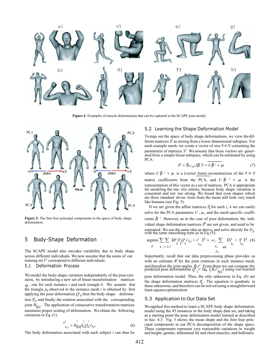
using the 70 training instances in our pose data set. Fig. 4
shows
examples of meshes that can be represented by our learned model.
Note that these examples do not correspond to meshes in the training
data set; they are new poses synthesized completely from a vector of
joint rotations R, using Eq. (3) to define the Q matrices, and Eq. (2)
to generate themesh.
The model captures well the shoulder deformations, the bulging
of the biceps and the twisting of the spine. It deals reasonably well
with the elbow and knee joints, although example (g) illustrates a
small amount of elbow smoothing that occurs in some poses. The
model exhibits an artifact in the armpit, which is caused by hole-
filling in the templatemesh.
Generating each mesh given the matrices takes
approximately
1 second, only 1.5 orders of magnitude away from real time, open-
ing the possibility of using this type of deformation model forreal-
time animation of synthesized or cached motion sequences.
411
�
Figure 4: Examples of muscle deformations that can be captured in the SCAPE pose model.
5.2 Learning the Shape Deformation Model
To map out the space of body shape deformations, we view thedif-
ferent matrices Si as arising from a lower dimensional subspace. For
each example mesh, we create a vector of size 9 × N containing the
parameters of matrices Si. We assume that these vectors are gener-
ated from a simple linear subspace, which can be estimated by using
PCA:
Si = SU,µ (β i) = Uβ i+µ
(7)
where U β i + µ is a (vector form) reconstruction of the 9 × N
matrix coefficients from the PCA, and U β i + µ is the
representation of this vector as a set of matrices. PCA is appropriate
for modeling the ma- trix entries, because body shape variation is
consistent and not
too strong. We found that even shapes which
are three standard devia- tions from the mean still look very much
like humans (see Fig. 5).
If we are given the affine matrices Si for each i, k we can easily
solve for the PCA parameters U , µ, and the mesh-specific coeffi-
cients β i. However, as in the case of pose deformation, the indi-
vidual shape deformation matrices Si are not given, and need to be
estimated. We use the same idea as above, and solve directly for Si ,
k
with the same smoothing term as in Eq.(5):
I2 + ws ISi − Si I2. (8)
argmin IRi Si Qi vˆk,j − vi
k,j
k k
k2
k1
k
k
k
Si
k j=2,3
adj
k1
,k2
k
k
k
f[k]
Importantly, recall that our data preprocessing phase provides us
with an estimate Ri for the joint rotations in each instance mesh,
and therefore the joint angles .6.ri. From these we can compute the
predicted pose deformations Qi = Qa (.6.ri
) using our learned
pose deformation model. Thus, the only unknowns in Eq. (8) are
the shape deformation matrices Si . The equation is quadratic in
these unknowns, and therefore can be solved using a straightforward
least-squaresoptimization.
5.3 Application to Our Data Set
Weapplied this method to learn a SCAPE body shape deformation
model using the 45 instances in the body shape data set, and taking
as a starting point the pose deformation model learned as described
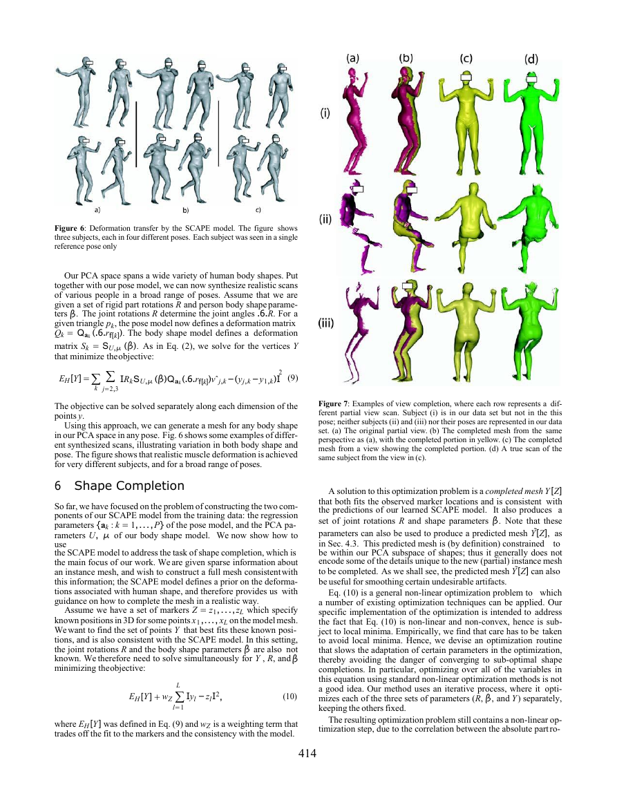
in Sec. 4.3. Fig. 5 shows the mean shape and the first four prin-
cipal components in our PCA decomposition of the shape space.
These components represent very reasonable variations in weight
and height, gender, abdominal fat and chest muscles, and bulkiness
Figure 5: The first four principal components in the space of body shape
deformation
5 Body-Shape Deformation
The SCAPE model also encodes variability due to body shape
across different individuals. We now assume that the scans of our
training set Y i correspond to different individuals.
5.1 Deformation Process
Wemodel the body-shape variation independently of the posevari-
ation, by introducing a new set of linear transformation matrices
k , one for each instance i and each triangle k. We assume that
Si
the triangle pk observed in the instance mesh i is obtained by first
applying the pose deformation Qi , then the body shape deforma-
tion Si , and finally the rotation associated with the corresponding
k
joint Ri
. The application of consecutive transformation matrices
maintains proper scaling of deformation. Weobtain the following
extension to Eq. (1):
f[k]
k
(6)
The body deformation associated with each subject i can thus be
i
vi
k, j = Rf[k]SkQkvˆk,j.
i
i
412
�
modeled as a set of matrices Si = {Si
k
: k = 1,...,P}.
of the chest versus thehips.
413
�
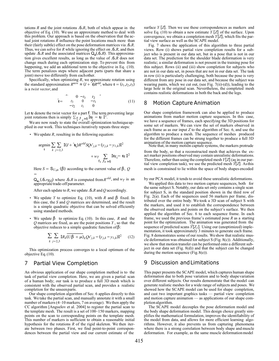
Figure 6: Deformation transfer by the SCAPE model. The figure shows
three subjects, each in four different poses. Each subject was seen in a single
reference pose only
Our PCA space spans a wide variety of human body shapes. Put
together with our pose model, we can now synthesize realistic scans
of various people in a broad range of poses. Assume that we are
given a set of rigid part rotations R and person body shapeparame-
ters β. The joint rotations R determine the joint angles .6.R. For a
given triangle pk, the pose model now defines a deformation matrix
Qk = Qak (.6.rf[k]). The body shape model defines a deformation
matrix Sk = SU,µ (β). As in Eq. (2), we solve for the vertices Y
that minimize theobjective:
EH[Y]=
k
j=2,3
2
IRkSU,µ (β)Qak(.6.rf[k])vˆj,k−(yj,k −y1,k)I
(9)
The objective can be solved separately along each dimension of the
points y.
Using this approach, we can generate a mesh for any body shape
in our PCA space in any pose. Fig. 6 shows some examples of differ-
ent synthesized scans, illustrating variation in both body shape and
pose. The figure shows that realistic muscle deformation is achieved
for very different subjects, and for a broad range of poses.
6 Shape Completion
So far, we have focused on the problem of constructing the two com-
ponents of our SCAPE model from the training data: the regression
parameters {ak : k = 1,...,P} of the pose model, and the PCA pa-
rameters U, µ of our body shape model. We now show how to
use
the SCAPE model to address the task of shape completion, which is
the main focus of our work. We are given sparse information about
an instance mesh, and wish to construct a full mesh consistentwith
this information; the SCAPE model defines a prior on the deforma-
tions associated with human shape, and therefore provides us with
guidance on how to complete the mesh in a realistic way.
Assume we have a set of markers Z = z1,...,zL which specify
known positions in 3D for some points x1,..., xL on the model mesh.
Wewant to find the set of points Y that best fits these known posi-
tions, and is also consistent with the SCAPE model. In this setting,
the joint rotations R and the body shape parameters β are also not
known. We therefore need to solve simultaneously for Y , R, andβ
minimizing theobjective:
EH[Y]+ wZ Iyl − zlI2,
L
l=1
(10)
where EH[Y] was defined in Eq. (9) and wZ is a weighting term that
trades off the fit to the markers and the consistency with the model.
414
Figure 7: Examples of view completion, where each row represents a dif-
ferent partial view scan. Subject (i) is in our data set but not in the this
pose; neither subjects (ii) and (iii) nor their poses are represented in our data
set. (a) The original partial view. (b) The completed mesh from the same
perspective as (a), with the completed portion in yellow. (c) The completed
mesh from a view showing the completed portion. (d) A true scan of the
same subject from the view in (c).
A solution to this optimization problem is a completed mesh Y[Z]
that both fits the observed marker locations and is consistent with
the predictions of our learned SCAPE model. It also produces a
set of joint rotations R and shape parameters β. Note that these
parameters can also be used to produce a predicted mesh Y˜[Z], as
in Sec. 4.3. This predicted mesh is (by definition) constrained to
be within our PCA subspace of shapes; thus it generally does not
encode some of the details unique to the new (partial) instance mesh
to be completed. As we shall see, the predicted mesh Y˜[Z] can also
be useful for smoothing certain undesirable artifacts.
Eq. (10) is a general non-linear optimization problem to which
a number of existing optimization techniques can be applied. Our
specific implementation of the optimization is intended to address
the fact that Eq. (10) is non-linear and non-convex, hence is sub-
ject to local minima. Empirically, we find that care has to be taken
to avoid local minima. Hence, we devise an optimization routine
that slows the adaptation of certain parameters in the optimization,
thereby avoiding the danger of converging to sub-optimal shape
completions. In particular, optimizing over all of the variables in
this equation using standard non-linear optimization methods is not
a good idea. Our method uses an iterative process, where it opti-
mizes each of the three sets of parameters (R, β, and Y) separately,
keeping the others fixed.
The resulting optimization problem still contains a non-linear op-
timization step, due to the correlation between the absolute partro-
�
tations R and the joint rotations .6.R, both of which appear in the
objective of Eq. (10). We use an approximate method to deal with
this problem. Our approach is based on the observation that the ac-
tual joint rotations R influence the point locations much more than
their (fairly subtle) effect on the pose deformation matrices via .6.R.
Thus, we can solve for R while ignoring the effect on .6.R, and then
update .6.R and the associated matrices Qa(.6.R). This approxima-
tion gives excellent results, as long as the value of .6.R does not
change much during each optimization step. To prevent this from
happening, we add an additional term to the objective in Eq. (10).
The term penalizes steps where adjacent parts (parts that share a
joint) move too differently from eachother.
Specifically, when optimizing R, we approximate rotation using
the standard approximation Rnew ≈ (I + ˆt)Rold, where t = (t1,t2,t3)
is a twist vector, and
ˆt=
I 0 −t3
0
t1
t3
−t2
1
t2
−t1
0
(11)
Let tf denote the twist vector for a part f. The term preventing large
joint rotations then is simply ∑f ,f
1
We are now ready to state the overall optimization techniqueap-
plied in our work. This techniques iteratively repeats three steps:
adj Itf − tf I2.
1
2
2
• We update R, resulting in the following equation:
argmin I(I+ˆtfk)RoldSQvˆj,k −(y j,k − y1,k)I2
t
k j=2,3
+wT
f1 ,f2 adj
Itf − tf I2
1
2
Here S = SU,µ (β) according to the current value of β, Q
=
Qak(.6.rf[k]) where .6.R is computed fromR
appropriatetrade-offparameter.
After each update to R, we update .6.R and Q accordingly.
old, and wT is an
• We update Y to optimize Eq. (10), with R and β fixed. In
this case, the S and Q matrices are determined, and the result
is a simple quadratic objective that can be solved efficiently
using standard methods.
• We update β to optimize Eq. (10). In this case, R and the
Q matrices are fixed, as are the point positions Y , so that the
objective reduces to a simple quadratic function ofβ:
IRk(Uβ +µ)kQvˆj,k −(y j,k −y1,k)I2
(12)
k j=2,3
This optimization process converges to a local optimum of the
objective Eq.(10).
7 Partial View Completion
An obvious application of our shape completion method is to the
task of partial view completion. Here, we are given a partial scan
of a human body; our task is to produce a full 3D mesh which is
consistent with the observed partial scan, and provides a realistic
completion for the unseenparts.
Our shape completion algorithm of Sec. 6 applies directly to this
task. We take the partial scan, and manually annotate it with a small
number of markers (4–10 markers, 7 on average). We then apply the
CC algorithm [Anguelov et al. 2004] to register the partial scan to
the template mesh. The result is a set of 100–150 markers, mapping
points on the scan to corresponding points on the template mesh.
This number of markers is sufficient to obtain a reasonable initial
hypothesis for the rotations R of the rigid skeleton. We then iter-
ate between two phases. First, we find point-to-point correspon-
dences between the partial view and our current estimate of the
surface Y [Z]. Then we use these correspondences as markers and
solve Eq. (10) to obtain a new estimate Y [Z] of the surface. Upon
convergence, we obtain a completion mesh Y[Z], which fits the par-
tial view surface as well as the SCAPE model.
Fig. 7 shows the application of this algorithm to three partial
views. Row (i) shows partial view completion results for a sub-
ject who is present in our data set, but in a pose that is not in our
data set. The prediction for the shoulder blade deformation is very
realistic; a similar deformation is not present in the training pose for
this subject. Rows (ii) and (iii) show completion for subjects who
are not in our data set, in poses that are not in our data set. The task
in row (ii) is particularly challenging, both because the pose is very
different from any pose in our data set, and because the subject was
wearing pants, which we cut out, (see Fig. 7(ii)-(d)), leading to the
large hole in the original scan. Nevertheless, the completed mesh
contains realistic deformations in both the back and the legs.
8 Motion Capture Animation
Our shape completion framework can also be applied to produce
animations from marker motion capture sequences. In this case,
we have a sequence of frames, each specifying the 3D positions for
some set of markers. We can view the set of markers observed in
each frame as as our input Z to the algorithm of Sec. 6, and use the
algorithm to produce a mesh. The sequence of meshes produced
for the different frames can be strung together to produce a full 3D
animation of the motion capture sequence.
Note that, in many motion capture systems, the markers protrude
from the body, so that a reconstructed mesh that achieves the ex-
act marker positions observed may contain unrealistic deformations.
Therefore, rather than using the completed mesh Y[Z] (as in our par-
tial view completion task), we use the predicted mesh Y˜[Z]. Asthis
mesh is constrained to lie within the space of body shapes encoded
by our PCA model, it tends to avoid these unrealistic deformations.
We applied this data to two motion capture sequences, both for
the same subject S. Notably, our data set only contains a single scan
for subject S, in the standard position shown in the third row of
Fig. 2(a). Each of the sequences used 56 markers per frame, dis-
tributed over the entire body. We took a 3D scan of subject S with
the markers, and used it to establish the correspondence between
the observed markers and points on the subject’s surface. We then
applied the algorithm of Sec. 6 to each sequence frame. In each
frame, we used the previous frame’s estimated pose R as a starting
point for the optimization. The animation was generated from the
sequence of predicted scans Y˜[Zf]. Using our (unoptimized) imple-
mentation, it took approximately 3 minutes to generate each frame.
Fig. 8 demonstrates some of our results. Weshow that realistic mus-
cle deformation was obtained for subject S (Fig. 8(c)). Additionally,
we show that motion transfer can be performed onto a different sub-
ject in our data set (Fig. 8(d)) and that the subject can be changed
during the motion sequence (Fig.8(e)).
9 Discussion andLimitations
This paper presents the SCAPE model, which captures human shape
deformation due to both pose variation and to body shapevariation
over different subjects. Our results demonstrate that the model can
generate realistic meshes for a wide range of subjects and poses. We
showed how the SCAPE model can be used for shape completion,
and cast two important graphics tasks — partial view completion
and motion capture animation — as applications of our shape com-
pletionalgorithm.
The SCAPE model decouples the pose deformation model and
the body shape deformation model. This design choice greatly sim-
plifies the mathematical formulation, improves the identifiability of
the model from data, and allows for more efficient learning algo-
rithms. However, it also prevents us from capturing phenomena
where there is a strong correlation between body shape and muscle
deformation. For example, as the same muscle deformationmodel
415
�





 2023年江西萍乡中考道德与法治真题及答案.doc
 2012年重庆南川中考生物真题及答案.doc
 2013年江西师范大学地理学综合及文艺理论基础考研真题.doc
 2020年四川甘孜小升初语文真题及答案I卷.doc
 2020年注册岩土工程师专业基础考试真题及答案.doc
 2023-2024学年福建省厦门市九年级上学期数学月考试题及答案.doc
 2021-2022学年辽宁省沈阳市大东区九年级上学期语文期末试题及答案.doc
 2022-2023学年北京东城区初三第一学期物理期末试卷及答案.doc
 2018上半年江西教师资格初中地理学科知识与教学能力真题及答案.doc
 2012年河北国家公务员申论考试真题及答案-省级.doc
 2020-2021学年江苏省扬州市江都区邵樊片九年级上学期数学第一次质量检测试题及答案.doc
 2022下半年黑龙江教师资格证中学综合素质真题及答案.doc