Recognizing Human Actions from Still Images with Latent Poses
Weilong Yang, Yang Wang, and Greg Mori
School of Computing Science
Simon Fraser University
Burnaby, BC, Canada
wya16@sfu.ca, ywang12@cs.sfu.ca, mori@cs.sfu.ca
Abstract
We consider the problem of recognizing human actions
from still images. We propose a novel approach that treats
the pose of the person in the image as latent variables
that will help with recognition. Different from other work
that learns separate systems for pose estimation and action
recognition, then combines them in an ad-hoc fashion, our
system is trained in an integrated fashion that jointly con-
siders poses and actions. Our learning objective is designed
to directly exploit the pose information for action recogni-
tion. Our experimental results demonstrate that by inferring
the latent poses, we can improve the final action recognition
results.
1. Introduction
Consider the two images shown in Fig. 1(left). Even
though only still images are given, we as humans can still
perceive the actions (walking, playing golf) conveyed by
those images. The primary goal of this work is to recognize
actions from still images. In still images, the information
about the action label of an image mainly comes from the
pose, i.e. the configuration of body parts, of the person in
the image. However, not all body parts are equally impor-
tant for differentiating various actions. Consider the poses
shown in Fig. 1(middle). The configurations of torso, head
and legs are quite similar for both walking and playing golf.
The main difference for these two actions in terms of the
pose is the configuration of the arms. For example, “playing
golf” seems to have very distinctive V-shaped arms, while
“walking” seems to have two arms hanging on the side. A
standard pose estimator tries to find the correct locations of
all the body parts. The novelty of our work is that we do
not need to correctly infer complete pose configuration in
order to do action recognition. In the example of “walking”
versus “playing golf”, as long as we get correct locations of
the arms, we can correctly recognize the action, even if the
locations of other body parts are incorrect. The challenge is
Figure 1. Illustration of our proposed approach. Our goal is to infer
the action label of a still image. We treat the pose of the person
in the image as “latent variables” in our system. The “pose” is
learned in a way that is directly tied to action classification.
how to learn a system that is aware of the importance of dif-
ferent body parts, so it can focus on the arms when trying to
differentiate between “walking” and “playing golf”. We in-
troduce a novel model that jointly learns poses and actions
in a principled framework.
Human action recognition is an extremely important
and active research area in computer vision, due to its
wide range of applications, e.g. surveillance, entertainment,
human-computer interaction, image and video search, etc.
Space constraints do not allow an extensive review of the
field, but a comprehensive survey is available in [9]. Most
of the work in this field focuses on recognizing actions from
videos [13, 15, 18] using motion cues, and a significant
amount of progress has been made in the past few years.
Action recognition from still images, on the other hand, has
not been widely studied. We believe analyzing actions from
still images is important. Progress made here can be directly
applied to videos. There are also applications that directly
require understanding still images of human actions, e.g.
news/sports image retrieval and analysis.
Not surprisingly, recognizing human actions from still
images is considerably more challenging than video se-
1
�
quences. In videos, the motion cue provides a rich source of
information for differentiating various actions. But in still
images, the only information we can rely on is the shape (or
the pose) of the person in an image. Previous work mainly
focuses on building good representations for shapes and
poses of people in images. Wang et al. [20] cluster different
human poses using distances calculated from deformable
shape matching. Thurau and Hlav´aˇc [19] represent ac-
tions using histograms of pose primitives computed by non-
negative matrix factorization. Ikizler et al. [10] recognize
actions using a descriptor based on histograms of oriented
rectangles. Ikizler-Cinbis et al. [11] learn actions from web
images using HOG descriptors [3]. A limitation of these
approaches is that they all assume an image representation
based on global templates, i.e. an image is represented by
a feature descriptor extracted from the whole image. This
representation has been made popular due to its success in
pedestrian detection, in particular the work on histogram of
oriented gradient (HOG) by Dalal and Triggs [3]. This rep-
resentation might be appropriate for pedestrian detection,
since most pedestrians are upright. So it might be helpful
to represent all the pedestrians using a global template. But
when it comes to action recognition, global templates are
not flexible enough to represent the huge amount of varia-
tions for an action. For example, consider the images of the
“playing golf” action in Fig. 4. It is hard to imagine that a
single global template can capture all the pose variations of
this action. Recently, Felzenszwalb et al. [6] show that part-
based representations can better capture the pose variations
of an object, hence outperform global template representa-
tions. In this paper, we operationalize on the same intuition
and demonstrate that part-based representations are useful
for action recognition in still images as well. A major dif-
ference of our work from [6] is that we have ground-truth
labeling of the pose on the training data, i.e. our “parts” are
semantically meaningful.
Another important goal of this paper is to bridge the gap
between human action recognition and human pose esti-
mation. Those are two closely related research problems.
If we can reliably estimate the pose of a person, we can
use this information to recognize the action. However, in
the literature, they are typically touted as two separate re-
search problems and there has been only very little work
on combining them together. There is some work on trying
to combine these two problems in a cascade way, e.g. by
building an action recognition system on top of the output
of a pose estimation system. For example, Ramanan and
Forsyth [17] annotate and synthesize human actions in 3D
by track people in 2D and match the track to an annotated
motion capture dataset. Their work uses videos rather than
still images, but the general idea is similar. Ferrari et al. [8]
retrieve TV shots containing a particular 2D human pose by
first estimating the human pose, then searching shots based
Figure 2. Difference between previous work and ours. (Top) Pre-
vious work typically approaches pose estimation and action recog-
nition as two separate problems, and uses the output of the former
as the input to the latter. (Bottom) We treat pose estimation and
action recognition as an single problem, and learn everything in
an integrated framework.
on a feature vector extracted from the pose. But it has been
difficult to establish the value of pose estimation for action
recognition in this cascade manner, mainly because pose es-
timation is still a largely unsolved problem. It is question-
able whether the output of any pose estimation algorithm is
reliable enough to be directly used for action recognition.
In this paper, we propose a novel way of combining ac-
tion recognition and pose estimation together to achieve
the end goal of action recognition. Our work is different
from previous work in two perspectives. First, instead of
representing the human pose as the configuration of kine-
matic body parts [16], e.g. upper-limb, lower-limb, head,
etc., we choose to use an exemplar-based pose representa-
tion, “poselet”. This notation of “poselet” is first proposed
in [2] and used to denote a set of patches with similar 3D
pose configuration.
In this paper, for the purpose of ac-
tion recognition, we further restrict those patches not only
to have similar configuration, but also from the same action
class. Second, as illustrated by the diagram in Fig. 2 (top),
previous work typically treats pose estimation and action
recognition as two separate learning problems, and uses the
output of a pose estimation algorithm as the input of an ac-
tion recognition system [8, 10]. As pointed out earlier, the
problem with this approach is that the output of the pose es-
timation is typically not reliable. Instead, as illustrated by
the diagram in Fig. 2 (bottom), we treat pose estimation and
action recognition as two components of a single learning
problem, and jointly learn the whole system in an integrated
manner. But our learning objective is designed in a way that
allows pose information to help action classification.
The high-level idea of our proposed approach can be
seen from Fig. 1. Our goal is to infer the action label of a
still image. We treat the pose of the person as intermediate
information useful for recognizing the action. But instead
of trying to infer the pose correctly using a pose estimation
algorithm, we treat the pose as latent variables in the whole
system. Compared with previous work on exploiting pose
for recognition [17, 8], the “pose” in our system is learned
in a way that is directly tied to our end goal of action clas-
sification.
�
2. Pose Representation
In this paper, we treat human pose as latent information
and use it to assist the task of action recognition. Since
we do not aim to obtain good pose estimation results in the
end, the latent pose in our approach is not restricted to any
specific type of pose representation. Because our focus is
action recognition, we decide to choose a coarse exemplar-
based pose representation. It is an action-specific variant of
the “poselet” proposed in [2]. In this paper, we use the no-
tation of “poselet” to refer to a set of patches not only with
similar pose configuration, but also from the same action
class. Fig. 3 illustrates the four poselets of a walking image.
As we can see, the poselet normally covers more than one
semantically meaningful part in terms of limbs and thus it is
distinct from the background. So, the detection of poselets
is more reliable than limb detection, especially with clut-
tered backgrounds.
In [2], a dataset is built where the joint positions of each
human image are labeled in 3D space via a 2D-3D lifting
procedure. We simply annotate the joint positions of hu-
man body in the 2D image space, as shown in Fig. 4. From
the pose annotation, we can easily collect a set of patches
with similar pose configuration. Based on the intuition that
action-specific parts contain more discriminative informa-
tion, we decide to select the poselets per action. For ex-
ample, we would like to select a number of poselets from
running-legs, or walking arms. The procedure of poselet
selection for a particular action (e.g. running) is as follows:
1. We first divide the human pose annotation of the run-
ning images into four parts, legs, left-arm, right-arm, and
upper-body; 2. We cluster the joints on each part into sev-
eral clusters based their normalized x and y coordinates; 3.
We remove clusters with very few examples; 4. Based on
the pose clusters, we crop the corresponding patches from
the images and form a set of poselets for the running ac-
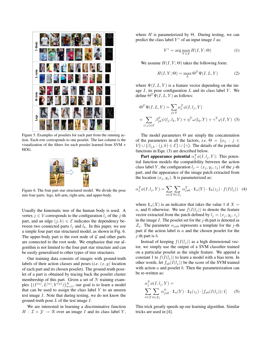
tion. Representative poselets from the running action are
shown in Fig. 5. As we can see, among each poselet the ap-
pearance of each patch looks different, but they have very
similar semantic meaning. As pointed in [2], this is also
one advantage of using poselets. We repeat this process for
other actions and obtain 90 poselets in total in the end.
In order to detect the presence of each poselet, we train a
classifier for each poselet. We use the standard linear SVM
and the histograms of Oriented Gradients feature proposed
by Dalal and Triggs [3]. The positive examples are the
patches from each poselet cluster. The negative examples
are randomly selected from images which have the different
action label to the positive examples. For example, when we
train the classifier for one of “running-legs” poselets, we se-
lect the negative examples from all other action categories
except for the running action. The learned running poselet
templates are visualized in the last column in Fig. 5.
Figure 3. Visualization of the poselets for a walking image.
Ground-truth skeleton is overlayed on image. Examples of pose-
lets for each part are shown.
(a)
(b)
(c)
(d)
(e)
Figure 4. Sample images of the still image action dataset [11], and
the ground truth pose annotation. The locations of 14 joints have
been annotated on each action image. (a) Running; (b) Walking;
(c) Playing Golf; (d) Sitting; (e) Dancing.
3. Model Formulation
Let I be an image containing a person.
In this paper,
we consider a figure-centric representation where I only
contains one person centered in the middle of the image.
This representation can be obtained from a standard pedes-
trian detection system. Let Y be the action label of the
person, and L be the pose of the person. We denote L as
L = (l0, l1, ..., lK−1), where K is the number of parts. In
this paper, we choose K = 4 corresponding to upper-body,
legs, left-arm, and right-arm. The configuration of the k-th
part lk is represented as lk = (xk, yk, zk), where (xk, yk)
indicates the (x, y) locations of the k-th part in the image,
and zk ∈ Zk is the index of the chosen poselet for the k-th
part. We have used Zk to denote the poselet set correspond-
ing to the part k. In this paper, we use |Zk| as 26, 20, 20, 24
for the four parts: legs, left-arm, right-arm, and upper-body,
based on our clustering results.
Similar to the standard pictorial structure models [7, 16]
in human pose estimation, we use an undirected graph
G = (V,E) to constrain the configuration of the pose L.
�
where H is parameterized by Θ. During testing, we can
predict the class label Y ∗ of an input image I as:
Y ∗ = arg max
Y ∈Y H(I, Y ; Θ)
We assume H(I, Y ; Θ) takes the following form:
H(I, Y ; Θ) = max
L
ΘT Ψ(I, L, Y )
(1)
(2)
where Ψ(I, L, Y ) is a feature vector depending on the im-
age I, its pose configuration L and its class label Y . We
define ΘT Ψ(I, L, Y ) as follows:
ΘT Ψ(I, L, Y ) =
+
j∈V
(i,j)∈E
j φ(I, lj, Y )
αT
jkψ(lj, lk, Y ) + ηT ω(l0, Y ) + γT ϕ(I, Y ) (3)
βT
Figure 5. Examples of poselets for each part from the running ac-
tion. Each row corresponds to one poselet. The last column is the
visualization of the filters for each poselet learned from SVM +
HOG.
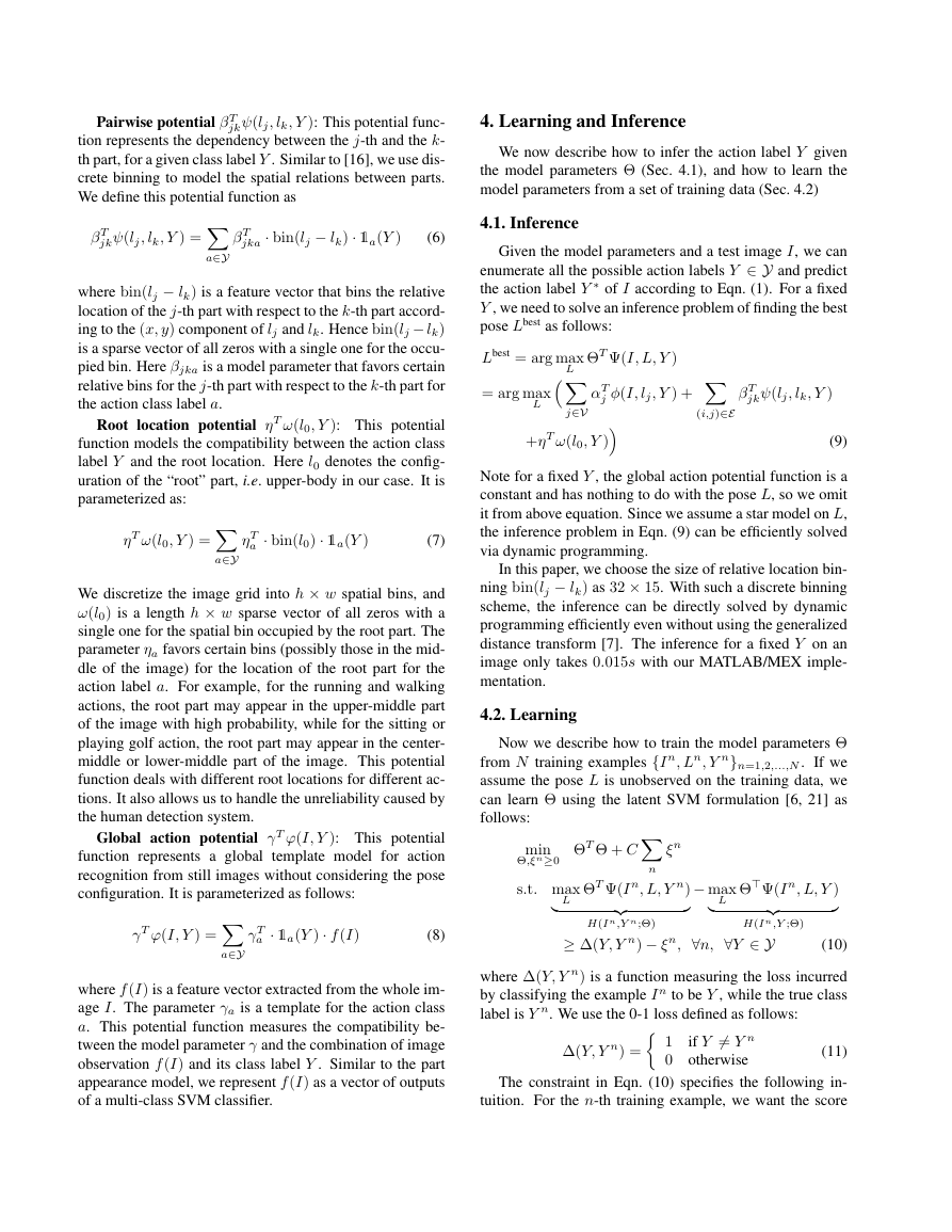
Figure 6. The four part star structured model. We divide the pose
into four parts: legs, left-arm, right-arm, and upper-body.
Usually the kinematic tree of the human body is used. A
vertex j ∈ V corresponds to the configuration lj of the j-th
part, and an edge (j, k) ∈ E indicates the dependency be-
tween two connected parts lj and lk. In this paper, we use
a simple four part star structured model, as shown in Fig. 6.
The upper-body part is the root node of G and other parts
are connected to the root node. We emphasize that our al-
gorithm is not limited to the four part star structure and can
be easily generalized to other types of tree structures.
Our training data consists of images with ground-truth
labels of their action classes and poses (i.e. (x, y) location
of each part and its chosen poselet). The ground-truth pose-
let of a part is obtained by tracing back the poselet cluster
membership of this part. Given a set of N training exam-
ples {(I (n), L(n), Y (n))}N
n=1, our goal is to learn a model
that can be used to assign the class label Y to an unseen
test image I. Note that during testing, we do not know the
ground-truth pose L of the test image I.
We are interested in learning a discriminative function
H : I × Y → R over an image I and its class label Y ,
The model parameters Θ are simply the concatenation
of the parameters in all the factors, i.e. Θ = {αj : j ∈
V} ∪ {βj,k : (j, k) ∈ E} ∪ {γ}. The details of the potential
functions in Eqn. (3) are described below.
Part appearance potential αT
j φ(I, lj, Y ): This poten-
tial function models the compatibility between the action
class label Y , the configuration lj = (xj, yj, zj) of the j-th
part, and the appearance of the image patch extracted from
the location (xj, yj). It is parameterized as:
j φ(I, lj, Y ) =
αT
a∈Y
b∈Zj
jab · 1a(Y ) · 1b(zj) · f(I(lj))
αT
(4)
where 1a(X) is an indicator that takes the value 1 if X =
a, and 0 otherwise. We use f(I(lj)) to denote the feature
vector extracted from the patch defined by lj = (xj, yj, zj)
in the image I. The poselet set for the j-th part is denoted as
Zj. The parameter αjab represents a template for the j-th
part if the action label is a and the chosen poselet for the
j-th part is b.
Instead of keeping f(I(lj)) as a high dimensional vec-
tor, we simply use the output of a SVM classifier trained
on a particular poselet as the single feature. We append a
constant 1 to f(I(lj)) to learn a model with a bias term. In
other words, let fab(I(lj)) be the score of the SVM trained
with action a and poselet b. Then the parameterization can
be re-written as:
j φ(I, lj, Y ) =
αT
a∈Y
b∈Zj
jab · 1a(Y ) · 1b(zj) · [fab(I(lj)); 1]
αT
(5)
This trick greatly speeds up our learning algorithm. Similar
tricks are used in [4].
�
Pairwise potential βT
jkψ(lj, lk, Y ): This potential func-
tion represents the dependency between the j-th and the k-
th part, for a given class label Y . Similar to [16], we use dis-
crete binning to model the spatial relations between parts.
We define this potential function as
jka · bin(lj − lk) · 1a(Y )
βT
(6)
jkψ(lj, lk, Y ) =
βT
a∈Y
where bin(lj − lk) is a feature vector that bins the relative
location of the j-th part with respect to the k-th part accord-
ing to the (x, y) component of lj and lk. Hence bin(lj − lk)
is a sparse vector of all zeros with a single one for the occu-
pied bin. Here βjka is a model parameter that favors certain
relative bins for the j-th part with respect to the k-th part for
the action class label a.
Root location potential ηT ω(l0, Y ): This potential
function models the compatibility between the action class
label Y and the root location. Here l0 denotes the config-
uration of the “root” part, i.e. upper-body in our case. It is
parameterized as:
a · bin(l0) · 1a(Y )
ηT
(7)
ηT ω(l0, Y ) =
a∈Y
We discretize the image grid into h × w spatial bins, and
ω(l0) is a length h × w sparse vector of all zeros with a
single one for the spatial bin occupied by the root part. The
parameter ηa favors certain bins (possibly those in the mid-
dle of the image) for the location of the root part for the
action label a. For example, for the running and walking
actions, the root part may appear in the upper-middle part
of the image with high probability, while for the sitting or
playing golf action, the root part may appear in the center-
middle or lower-middle part of the image. This potential
function deals with different root locations for different ac-
tions. It also allows us to handle the unreliability caused by
the human detection system.
Global action potential γT ϕ(I, Y ): This potential
function represents a global template model for action
recognition from still images without considering the pose
configuration. It is parameterized as follows:
a · 1a(Y ) · f(I)
γT
γT ϕ(I, Y ) =
(8)
a∈Y
where f(I) is a feature vector extracted from the whole im-
age I. The parameter γa is a template for the action class
a. This potential function measures the compatibility be-
tween the model parameter γ and the combination of image
observation f(I) and its class label Y . Similar to the part
appearance model, we represent f(I) as a vector of outputs
of a multi-class SVM classifier.
4. Learning and Inference
We now describe how to infer the action label Y given
the model parameters Θ (Sec. 4.1), and how to learn the
model parameters from a set of training data (Sec. 4.2)
4.1. Inference
Given the model parameters and a test image I, we can
enumerate all the possible action labels Y ∈ Y and predict
the action label Y ∗ of I according to Eqn. (1). For a fixed
Y , we need to solve an inference problem of finding the best
pose Lbest as follows:
Lbest = arg max
= arg max
L
L
j∈V
ΘT Ψ(I, L, Y )
j φ(I, lj, Y ) +
αT
(i,j)∈E
+ηT ω(l0, Y )
jkψ(lj, lk, Y )
βT
(9)
Note for a fixed Y , the global action potential function is a
constant and has nothing to do with the pose L, so we omit
it from above equation. Since we assume a star model on L,
the inference problem in Eqn. (9) can be efficiently solved
via dynamic programming.
In this paper, we choose the size of relative location bin-
ning bin(lj − lk) as 32 × 15. With such a discrete binning
scheme, the inference can be directly solved by dynamic
programming efficiently even without using the generalized
distance transform [7]. The inference for a fixed Y on an
image only takes 0.015s with our MATLAB/MEX imple-
mentation.
4.2. Learning
Now we describe how to train the model parameters Θ
from N training examples {I n, Ln, Y n}n=1,2,...,N . If we
assume the pose L is unobserved on the training data, we
can learn Θ using the latent SVM formulation [6, 21] as
follows:
min
Θ,ξn≥0
ΘT Θ + C
ξn
s.t. max
ΘT Ψ(I n, L, Y n)
− max
ΘΨ(I n, L, Y )
L
L
H(I n,Y n;Θ)
≥ ∆(Y, Y n) − ξn, ∀n, ∀Y ∈ Y
H(I n,Y ;Θ)
(10)
n
where ∆(Y, Y n) is a function measuring the loss incurred
by classifying the example I n to be Y , while the true class
label is Y n. We use the 0-1 loss defined as follows:
∆(Y, Y n) =
(11)
The constraint in Eqn. (10) specifies the following in-
tuition. For the n-th training example, we want the score
1
if Y = Y n
0 otherwise
�
H(I n, Y ; Θ) = arg maxL ΘT Ψ(I n, L, Y ) to be high when
Y is the true class label, i.e. Y = Y n. In particular, we want
the score H(I n, Y n; Θ) to be higher than the score associ-
ated with any hypothesized class label H(I n, Y ; Θ) by 1 if
Y = Y n.
Now since L is observed on training data, one possi-
ble way to learn Θ is to plug-in the ground-truth pose in
Eqn. (10), i.e. optimize the following problem:
ΘT Θ + C
min
Θ,ξn≥0
s.t. ΘT Ψ(I n, Ln, Y n) − max
ξn
n
ΘΨ(I n, L, Y )
≥ ∆(Y, Y n) − ξn, ∀n, ∀Y ∈ Y
L
(12)
Our initial attempt of using Eqn. (12) suggests it does not
perform as well as Eqn. (10). We believe it is because the
learning objective in Eqn. (12) assumes that we will have
access to the correct pose estimation at run-time. This is
unrealistic. On the other hand, the learning objective in
Eqn. (10) mimics the situation at run-time, when we are
faced with a new image without the ground-truth pose. So
we will use the formulation in Eqn. (10) from now on. But
we would like to point out that Eqn. (10) does not ignore the
ground-truth pose information on the training data. That in-
formation has been implicitly built into the features which
are represented as outputs of SVM classifiers. Those SVM
classifiers are learned using the ground-truth information of
the pose on the training data.
The training problem in Eqn. (10) can be solved by the
non-convex cutting plane algorithm in [5], which is an ex-
tension of the popular convex cutting plane algorithm [12]
for learning structural SVM [1]. We briefly outline the al-
gorithm here.
Consider the following unconstrained formulation which
is equivalent to Eqn. (10):
Θ = arg min
Θ
ΘT Θ + C
Rn(Θ) where
Rn(Θ) = max
(∆(Y, Y n) + H(I n, Y ; Θ))
Y
−H(I n, Y n; Θ)
(13)
In a nutshell,
∂Θ (
∂Θ (
the learning algorithm in [5] itera-
tively builds an increasingly accurate piecewise quadratic
approximation of Eqn. (13) based on the subgradient
n Rn(Θ)).
It can be shown that the subgradient
n Rn(Θ)) is related to the most-violated constraint
of Eqn. (10). So in essence, the algorithm iteratively adds
the most-violated constraint of Eqn. (10) and solves a piece-
wise quadratic approximation at each iteration. It has been
proved that only a small number of constraints are needed
in order to achieve an reasonably accurate approximation to
the original problem [1].
n
Now the key issue is how to compute the subgradient
∂Θ (
n Rn(Θ)). Since
=
∂Θ
Rn(Θ)
∂ΘRn(Θ)
(14)
n
n
all we need to do it to figure out how to compute ∂ΘRn(Θ).
Let us define:
∆(Y, Y n) + ΘT Ψ(I n, L, Y ) (15)
Y,L
(Y ∗, L∗) = arg max
ΘT Ψ(I n, L, Y n)
L = arg max
∂ΘRn(Θ) = Ψ(I n, L∗, Y ∗) − Ψ(I n,L, Y n)
It can be shown that ∂ΘRn(Θ) can be calculated as
L
(16)
(17)
The calculation of the subgradient ∂ΘRn(Θ) involves solv-
ing two inference problems in Eqn. (15,16). As men-
tion in Sec. 4.1, the inference on arg maxL can be effi-
ciently solved via dynamic programming. The inference on
arg maxY is easy too, since the number of possible choices
of Y is small (e.g. |Y| = 5 in our case). So we can simply
enumerate all possible Y ∈ Y.
5. Experiments
We first test our algorithm on the still image action
dataset collected by Ikizler-Cinbis et al. [11]. This dataset
consists of still images from five action categories: running,
walking, playing golf, sitting, and dancing. The images of
this dataset are downloaded from the Internet. So there are
a lot of pose variations and cluttered backgrounds in the
dataset. In total, there are 2458 images in the dataset. We
further increase the size and pose variability of the dataset
by mirror-flipping all the images. Most of actions in the
dataset do not have axial symmetry. For example, running-
to-left and running-to-right appear very different in the im-
age. So mirror-flipping makes the dataset more diverse. We
manually annotate the pose with 14 joints on the human
body on all the images in the dataset, as shown in Fig. 41.
We select 1/3 of the images from each action category to
form the training set, and the rest of the images are used for
testing. We also ensure the testing set does not contain the
mirror-flipped version of any training image. Since we fo-
cus on action classification rather than human detection, we
simply normalize each image into the same size and put the
human figure in the center of the image, based on the pose
annotation information.
At the training stage, we create 90 poselets in total from
the training set following the method described in Sec-
tion 2. For each poselet, we train an SVM classifier based
on the HOG descriptors extracted from image patches at
1The
(http://www.sfu.ca/∼wya16/latent/latentpose.html)
annotations
are
available
online
�
(a)
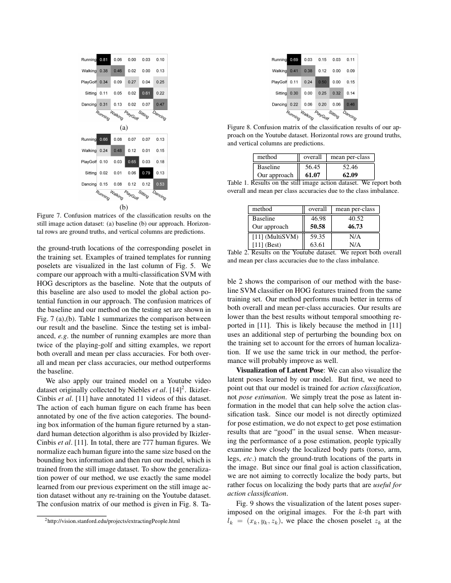
Figure 8. Confusion matrix of the classification results of our ap-
proach on the Youtube dataset. Horizontal rows are ground truths,
and vertical columns are predictions.
method
Baseline
Our approach
overall mean per-class
56.45
61.07
52.46
62.09
Table 1. Results on the still image action dataset. We report both
overall and mean per class accuracies due to the class imbalance.
(b)
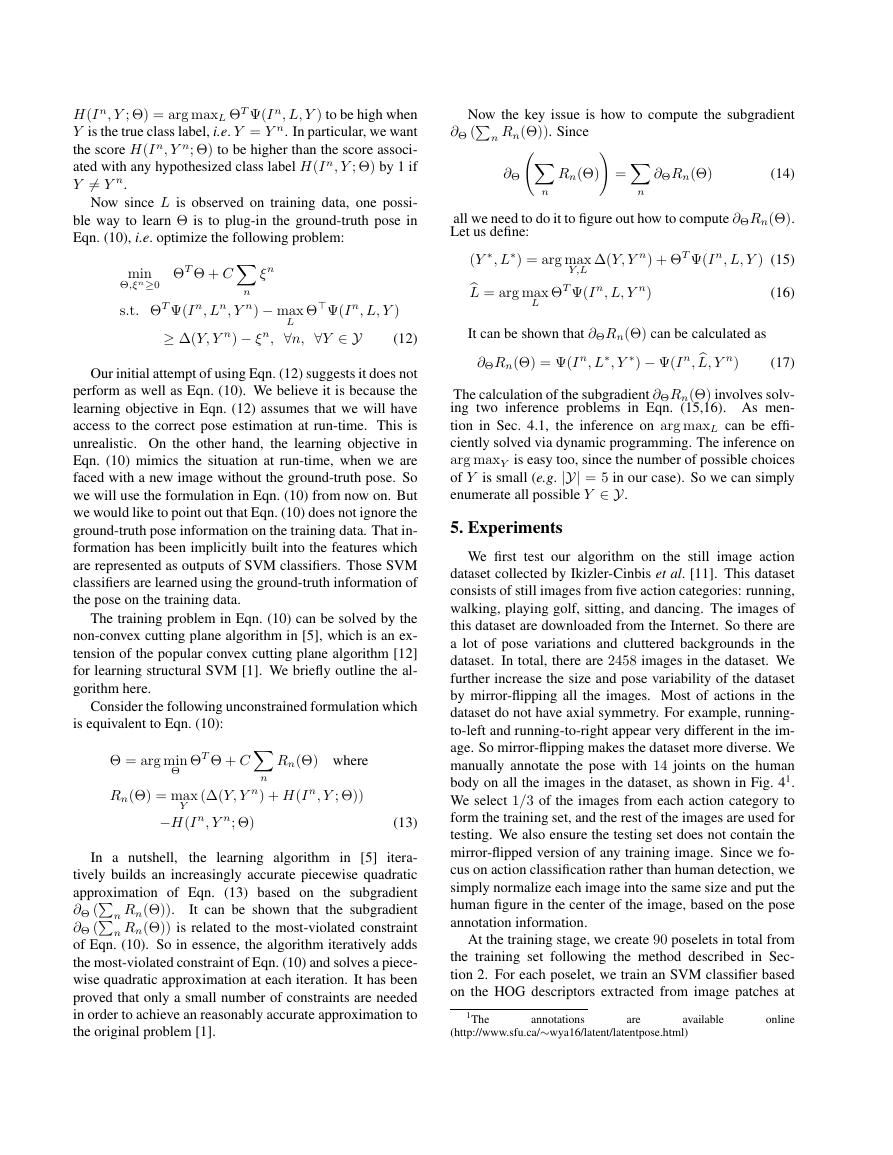
Figure 7. Confusion matrices of the classification results on the
still image action dataset: (a) baseline (b) our approach. Horizon-
tal rows are ground truths, and vertical columns are predictions.
the ground-truth locations of the corresponding poselet in
the training set. Examples of trained templates for running
poselets are visualized in the last column of Fig. 5. We
compare our approach with a multi-classification SVM with
HOG descriptors as the baseline. Note that the outputs of
this baseline are also used to model the global action po-
tential function in our approach. The confusion matrices of
the baseline and our method on the testing set are shown in
Fig. 7 (a),(b). Table 1 summarizes the comparison between
our result and the baseline. Since the testing set is imbal-
anced, e.g. the number of running examples are more than
twice of the playing-golf and sitting examples, we report
both overall and mean per class accuracies. For both over-
all and mean per class accuracies, our method outperforms
the baseline.
We also apply our trained model on a Youtube video
dataset originally collected by Niebles et al. [14]2. Ikizler-
Cinbis et al. [11] have annotated 11 videos of this dataset.
The action of each human figure on each frame has been
annotated by one of the five action categories. The bound-
ing box information of the human figure returned by a stan-
dard human detection algorithm is also provided by Ikizler-
Cinbis et al. [11]. In total, there are 777 human figures. We
normalize each human figure into the same size based on the
bounding box information and then run our model, which is
trained from the still image dataset. To show the generaliza-
tion power of our method, we use exactly the same model
learned from our previous experiment on the still image ac-
tion dataset without any re-training on the Youtube dataset.
The confusion matrix of our method is given in Fig. 8. Ta-
2http://vision.stanford.edu/projects/extractingPeople.html
method
Baseline
Our approach
[11] (MultiSVM)
[11] (Best)
overall mean per-class
46.98
50.58
59.35
63.61
40.52
46.73
N/A
N/A
Table 2. Results on the Youtube dataset. We report both overall
and mean per class accuracies due to the class imbalance.
ble 2 shows the comparison of our method with the base-
line SVM classifier on HOG features trained from the same
training set. Our method performs much better in terms of
both overall and mean per-class accuracies. Our results are
lower than the best results without temporal smoothing re-
ported in [11]. This is likely because the method in [11]
uses an additional step of perturbing the bounding box on
the training set to account for the errors of human localiza-
tion. If we use the same trick in our method, the perfor-
mance will probably improve as well.
Visualization of Latent Pose: We can also visualize the
latent poses learned by our model. But first, we need to
point out that our model is trained for action classification,
not pose estimation. We simply treat the pose as latent in-
formation in the model that can help solve the action clas-
sification task. Since our model is not directly optimized
for pose estimation, we do not expect to get pose estimation
results that are “good” in the usual sense. When measur-
ing the performance of a pose estimation, people typically
examine how closely the localized body parts (torso, arm,
legs, etc.) match the ground-truth locations of the parts in
the image. But since our final goal is action classification,
we are not aiming to correctly localize the body parts, but
rather focus on localizing the body parts that are useful for
action classification.
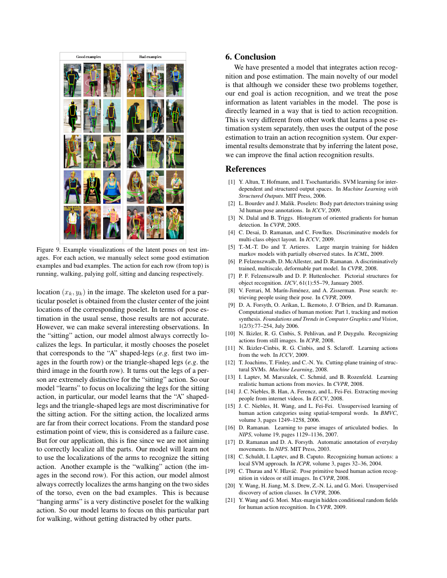
Fig. 9 shows the visualization of the latent poses super-
imposed on the original images. For the k-th part with
lk = (xk, yk, zk), we place the chosen poselet zk at the
�
6. Conclusion
We have presented a model that integrates action recog-
nition and pose estimation. The main novelty of our model
is that although we consider these two problems together,
our end goal is action recognition, and we treat the pose
information as latent variables in the model. The pose is
directly learned in a way that is tied to action recognition.
This is very different from other work that learns a pose es-
timation system separately, then uses the output of the pose
estimation to train an action recognition system. Our exper-
imental results demonstrate that by inferring the latent pose,
we can improve the final action recognition results.
References
[1] Y. Altun, T. Hofmann, and I. Tsochantaridis. SVM learning for inter-
dependent and structured output spaces. In Machine Learning with
Structured Outputs. MIT Press, 2006.
[2] L. Bourdev and J. Malik. Poselets: Body part detectors training using
3d human pose annotations. In ICCV, 2009.
[3] N. Dalal and B. Triggs. Histogram of oriented gradients for human
detection. In CVPR, 2005.
[4] C. Desai, D. Ramanan, and C. Fowlkes. Discriminative models for
multi-class object layout. In ICCV, 2009.
[5] T.-M.-T. Do and T. Artieres. Large margin training for hidden
markov models with partially observed states. In ICML, 2009.
[6] P. Felzenszwalb, D. McAllester, and D. Ramanan. A discriminatively
trained, multiscale, deformable part model. In CVPR, 2008.
[7] P. F. Felzenszwalb and D. P. Huttenlocher. Pictorial structures for
object recognition. IJCV, 61(1):55–79, January 2005.
[8] V. Ferrari, M. Mar´ın-Jim´enez, and A. Zisserman. Pose search: re-
trieving people using their pose. In CVPR, 2009.
[9] D. A. Forsyth, O. Arikan, L. Ikemoto, J. O’Brien, and D. Ramanan.
Computational studies of human motion: Part 1, tracking and motion
synthesis. Foundations and Trends in Computer Graphics and Vision,
1(2/3):77–254, July 2006.
[10] N. Ikizler, R. G. Cinbis, S. Pehlivan, and P. Duygulu. Recognizing
actions from still images. In ICPR, 2008.
[11] N. Ikizler-Cinbis, R. G. Cinbis, and S. Sclaroff. Learning actions
from the web. In ICCV, 2009.
[12] T. Joachims, T. Finley, and C.-N. Yu. Cutting-plane training of struc-
tural SVMs. Machine Learning, 2008.
[13] I. Laptev, M. Marszalek, C. Schmid, and B. Rozenfeld. Learning
realistic human actions from movies. In CVPR, 2008.
[14] J. C. Niebles, B. Han, A. Ferencz, and L. Fei-Fei. Extracting moving
people from internet videos. In ECCV, 2008.
[15] J. C. Niebles, H. Wang, and L. Fei-Fei. Unsupervised learning of
In BMVC,
human action categories using spatial-temporal words.
volume 3, pages 1249–1258, 2006.
[16] D. Ramanan. Learning to parse images of articulated bodies.
NIPS, volume 19, pages 1129–1136, 2007.
In
[17] D. Ramanan and D. A. Forsyth. Automatic annotation of everyday
movements. In NIPS. MIT Press, 2003.
[18] C. Schuldt, I. Laptev, and B. Caputo. Recognizing human actions: a
local SVM approach. In ICPR, volume 3, pages 32–36, 2004.
[19] C. Thurau and V. Hlav´aˇc. Pose primitive based human action recog-
nition in videos or still images. In CVPR, 2008.
[20] Y. Wang, H. Jiang, M. S. Drew, Z.-N. Li, and G. Mori. Unsupervised
discovery of action classes. In CVPR, 2006.
[21] Y. Wang and G. Mori. Max-margin hidden conditional random fields
for human action recognition. In CVPR, 2009.
Figure 9. Example visualizations of the latent poses on test im-
ages. For each action, we manually select some good estimation
examples and bad examples. The action for each row (from top) is
running, walking, palying golf, sitting and dancing respectively.
location (xk, yk) in the image. The skeleton used for a par-
ticular poselet is obtained from the cluster center of the joint
locations of the corresponding poselet. In terms of pose es-
timation in the usual sense, those results are not accurate.
However, we can make several interesting observations. In
the “sitting” action, our model almost always correctly lo-
calizes the legs. In particular, it mostly chooses the poselet
that corresponds to the “A” shaped-legs (e.g. first two im-
ages in the fourth row) or the triangle-shaped legs (e.g. the
third image in the fourth row). It turns out the legs of a per-
son are extremely distinctive for the “sitting” action. So our
model “learns” to focus on localizing the legs for the sitting
action, in particular, our model learns that the “A” shaped-
legs and the triangle-shaped legs are most discriminative for
the sitting action. For the sitting action, the localized arms
are far from their correct locations. From the standard pose
estimation point of view, this is considered as a failure case.
But for our application, this is fine since we are not aiming
to correctly localize all the parts. Our model will learn not
to use the localizations of the arms to recognize the sitting
action. Another example is the “walking” action (the im-
ages in the second row). For this action, our model almost
always correctly localizes the arms hanging on the two sides
of the torso, even on the bad examples. This is because
“hanging arms” is a very distinctive poselet for the walking
action. So our model learns to focus on this particular part
for walking, without getting distracted by other parts.
�




 2023年江西萍乡中考道德与法治真题及答案.doc
 2012年重庆南川中考生物真题及答案.doc
 2013年江西师范大学地理学综合及文艺理论基础考研真题.doc
 2020年四川甘孜小升初语文真题及答案I卷.doc
 2020年注册岩土工程师专业基础考试真题及答案.doc
 2023-2024学年福建省厦门市九年级上学期数学月考试题及答案.doc
 2021-2022学年辽宁省沈阳市大东区九年级上学期语文期末试题及答案.doc
 2022-2023学年北京东城区初三第一学期物理期末试卷及答案.doc
 2018上半年江西教师资格初中地理学科知识与教学能力真题及答案.doc
 2012年河北国家公务员申论考试真题及答案-省级.doc
 2020-2021学年江苏省扬州市江都区邵樊片九年级上学期数学第一次质量检测试题及答案.doc
 2022下半年黑龙江教师资格证中学综合素质真题及答案.doc