logo资料库

计算科学与工程Python简介Introduction to Python for Computational Science and Engineering.pdf

第1页 / 共170页
第2页 / 共170页
第3页 / 共170页
第4页 / 共170页
第5页 / 共170页
第6页 / 共170页
第7页 / 共170页
第8页 / 共170页
资料共170页,剩余部分请下载后查看
Introduction
Computational Modelling
Introduction
Computational Modelling
Programming to support computational modelling
Why Python for scientific computing?
Optimisation strategies
Get it right first, then make it fast
Prototyping in Python
Literature
Recorded video lectures on Python for beginners
Python tutor mailing list
Python version
These documents
Your feedback
A powerful calculator
Python prompt and Read-Eval-Print Loop (REPL)
Calculator
Integer division
How to avoid integer division
Why should I care about this division problem?
Mathematical functions
Variables
Terminology
Impossible equations
The += notation
Data Types and Data Structures
What type is it?
Numbers
Integers
Integer limits
Floating Point numbers
Complex numbers
Functions applicable to all types of numbers
Sequences
Sequence type 1: String
Sequence type 2: List
Sequence type 3: Tuples
Indexing sequences
Slicing sequences
Dictionaries
Passing arguments to functions
Call by value
Call by reference
Argument passing in Python
Performance considerations
Inadvertent modification of data
Copying objects
Equality and Identity/Sameness
Equality
Identity / Sameness
Example: Equality and identity
Introspection
dir()
Magic names
type
isinstance
help
Docstrings
Input and Output
Printing to standard output (normally the screen)
Simple print
Formatted printing
str and __str__
repr and __repr__
New-style string formatting
Changes from Python 2 to Python 3: print
Reading and writing files
File reading examples
Control Flow
Basics
Conditionals
If-then-else
For loop
While loop
Relational operators (comparisons) in if and while statements
Exceptions
Raising Exceptions
Creating our own exceptions
LBYL vs EAFP
Functions and modules
Introduction
Using functions
Defining functions
Default values and optional parameters
Modules
Importing modules
Creating modules
Use of __name__
Example 1
Example 2
Functional tools
Anonymous functions
Map
Filter
List comprehension
Reduce
Why not just use for-loops?
Speed
Common tasks
Many ways to compute a series
Sorting
Efficiency
From Matlab to Python
Important commands
The for-loop
The if-then statement
Indexing
Matrices
Python shells
IDLE
Python (command line)
Interactive Python (IPython)
IPython console
Jupyter Notebook
Spyder
Editors
Symbolic computation
SymPy
Output
Symbols
isympy
Numeric types
Differentiation and Integration
Ordinary differential equations
Series expansions and plotting
Linear equations and matrix inversion
Non linear equations
Output: LaTeX interface and pretty-printing
Automatic generation of C code
Related tools
Numerical Computation
Numbers and numbers
Limitations of number types
Using floating point numbers (carelessly)
Using floating point numbers carefully 1
Using floating point numbers carefully 2
Symbolic calculation
Summary
Exercise: infinite or finite loop
Numerical Python (numpy): arrays
Numpy introduction
History
Arrays
Convert from array to list or tuple
Standard Linear Algebra operations
More numpy examples…
Numpy for Matlab users
Visualising Data
Matplotlib (Pylab) – plotting y=f(x), (and a bit more)
Matplotlib and Pylab
First example
How to import matplotlib, pylab, pyplot, numpy and all that
IPython's inline mode
Saving the figure to a file
Interactive mode
Fine tuning your plot
Plotting more than one curve
Histograms
Visualising matrix data
Plots of z=f(x,y) and other features of Matplotlib
Visual Python
Basics, rotating and zooming
Setting the frame rate for animations
Tracking trajectories
Connecting objects (Cylinders, springs, …)
3d vision
Visualising higher dimensional data
Mayavi, Paraview, Visit
Writing vtk files from Python (pyvtk)
Numerical Methods using Python (scipy)
Overview
SciPy
Numerical integration
Exercise: integrate a function
Exercise: plot before you integrate
Solving ordinary differential equations
Exercise: using odeint
Root finding
Root finding using the bisection method
Exercise: root finding using the bisect method
Root finding using the fsolve funcion
Interpolation
Curve fitting
Fourier transforms
Optimisation
Other numerical methods
scipy.io: Scipy-input output
Where to go from here?
Advanced programming
Compiled programming language
Testing
Simulation models
Software engineering for research codes
Data and visualisation
Version control
Parallel execution
Acknowledgements
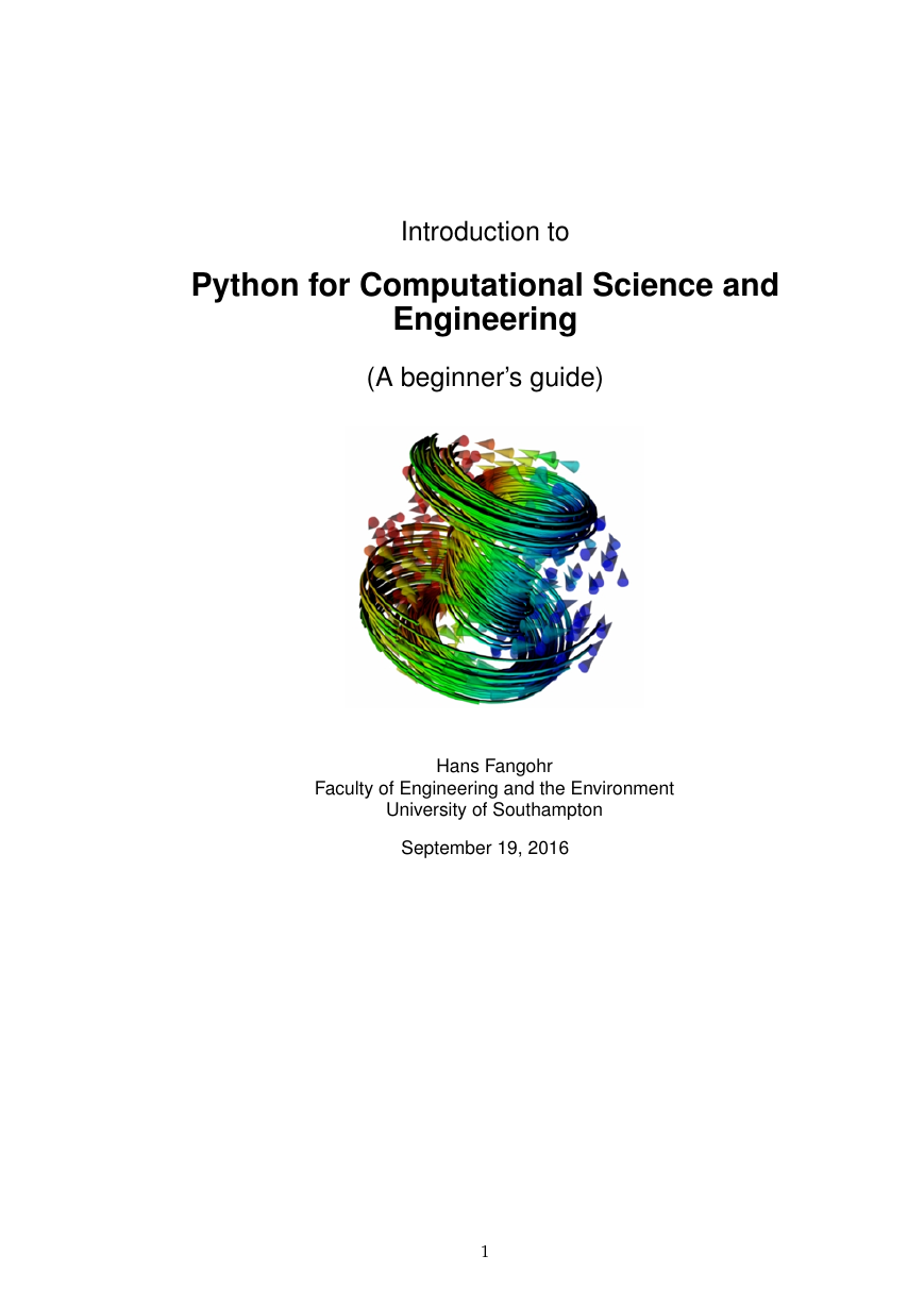
Introduction to Python for Computational Science and Engineering (A beginner’s guide) Hans Fangohr Faculty of Engineering and the Environment University of Southampton September 19, 2016 1
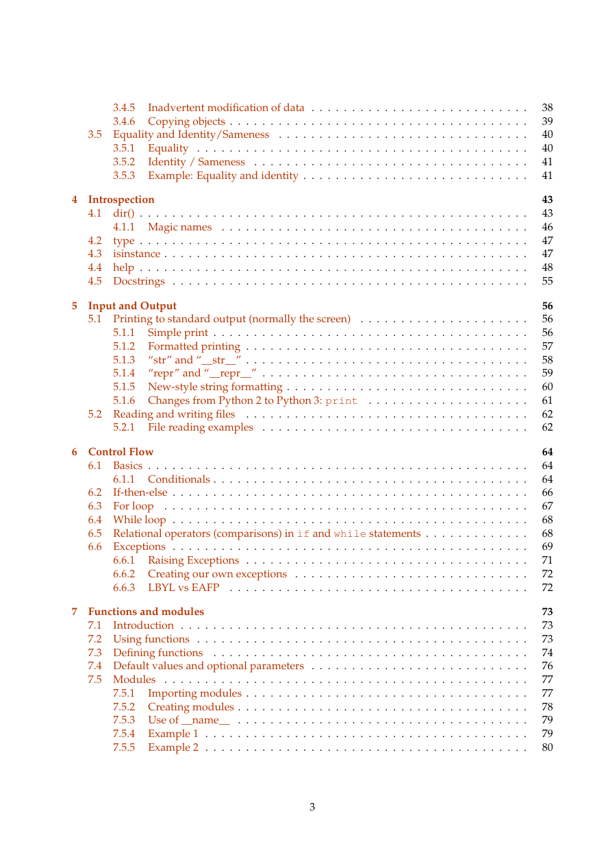
Contents 1 . . . Introduction 1.1 Computational Modelling . . Introduction . . . . . . . . . . . . . . . . . . . . . . . . . . . . . . . . . . 1.1.1 . . . . . . . . . . . . . . . . . . . . . . . . . . . . . . . . . 1.1.2 Computational Modelling . . . . . . . . . . . . . . . . . . . . . . . . . . . . . . 1.1.3 Programming to support computational modelling . . . . . . . . . . . . . . . 1.2 Why Python for scientific computing? . . . . . . . . . . . . . . . . . . . . . . . . . . . 1.2.1 Optimisation strategies . . . . . . . . . . . . . . . . . . . . . . . . . . . . . . . 1.2.2 Get it right first, then make it fast . . . . . . . . . . . . . . . . . . . . . . . . . . 1.2.3 Prototyping in Python . . . . . . . . . . . . . . . . . . . . . . . . . . . . . . . . . . . . . . . . . . . . . . . . . . . . . . . . . . . . . . . . . 1.3.1 Recorded video lectures on Python for beginners . . . . . . . . . . . . . . . . 1.3.2 Python tutor mailing list . . . . . . . . . . . . . . . . . . . . . . . . . . . . . . . . . . . . . . . . . . . . . . . . . . . . . . . . . . . . . . . . . . . . . . . . . . . . . . . . . . . . . . . . . . . . . . . . . . . . . . . . . . . . . . . . . . . . . . . . . . . . . . . . . . . . . 1.4 Python version . . 1.5 These documents . 1.6 Your feedback . . 1.3 Literature . . . . . . . . . . . . . . . . . . . . . . . . 2 A powerful calculator . . . . . . . . . . . . . 2.1 Python prompt and Read-Eval-Print Loop (REPL) 2.2 Calculator 2.3 . . . . . . . . . . . . . . . . . . . . . . . . . . . . . . . . . . . . . . . . . . . . . . . . . . . . . . . Integer division . . . . . . . . . . . . . . . . . . . . . . . . . . . . . . . . . . . 2.3.1 How to avoid integer division . . . . . . . . . . . . . . . . . . . . . . . . . . . 2.3.2 Why should I care about this division problem? . . . . . . . . . . . . . . . . . . . . . . . . . . . . . . . . . . . . . . . . . . . . . . . . . . . . . . . . . . . . . . . . . . . . . . . . . . . . . . . . . . . . . . . . . . . . . . . . . . . . . . . . . . . . . . . . . . . . . . . . . . . . . . . . . . . . . . . . . . . . . . . . . . . . . . . . . . . . . . . . . . . . . . . . . . . . . . . . . . . . . . . . . . 2.4 Mathematical functions . . 2.5 Variables . . . . 2.5.1 Terminology . . Impossible equations . . 2.6.1 The += notation . . . . . . 2.6 . . . . . . . . . . . . . . . . . . . . . 3.3 3 Data Types and Data Structures . . . . 3.1 What type is it? . 3.2 Numbers . . . . . . . . . . . . . . . . . . . . . . . . . . . . . . . . . . . . . . . . . . . . . . . . . . . . . . . . . . . . . . . . . . . . . . . . . . . . . . . . . . . . . . . . . . . . . . . . . . . . . . . . . . . . Integers . 3.2.1 Integer limits . . . . . . . . . . . . . . . . . . . . . . . . . . . . . . . . . . . 3.2.2 Floating Point numbers . . . . . . . . . . . . . . . . . . . . . . . . . . . . . . . 3.2.3 3.2.4 Complex numbers . . . . . . . . . . . . . . . . . . . . . . . . . . . . . . . . . . Functions applicable to all types of numbers . . . . . . . . . . . . . . . . . . . 3.2.5 Sequences . . . . . . . . . . . . . . . . . . . . . . . . . . . . . . . . Sequence type 1: String . . . . . . . . . . . . . . . . . . . . . . . . . . . . . . . 3.3.1 Sequence type 2: List . . . . . . . . . . . . . . . . . . . . . . . . . . . . . . . . . 3.3.2 Sequence type 3: Tuples . . . . . . . . . . . . . . . . . . . . . . . . . . . . . . . 3.3.3 Indexing sequences . 3.3.4 . . . . . . . . . . . . . . . . . . . . . . . . . . . . . . . . . . . . . . . . . . . . . . . . . . . . . . . . . . . . . . . . . . . 3.3.5 Slicing sequences . . . . . . . . . . . . . . . . . . . . . . . . . . . . . . . . . . . . 3.3.6 Dictionaries . 3.4 Passing arguments to functions . . . . . . . . . . . . . . . . . . . . . . . . . . . . . . . . . . . . . . . . . . . . . . . . . . . . . . . . . . . . . . . . . . 3.4.1 Call by value . 3.4.2 Call by reference . . . . . . . . . . . . . . . . . . . . . . . . . . . . . . . . . . . 3.4.3 Argument passing in Python . . . . . . . . . . . . . . . . . . . . . . . . . . . . 3.4.4 Performance considerations . . . . . . . . . . . . . . . . . . . . . . . . . . . . . . . . . . . . . . . . 7 7 7 7 8 8 10 10 10 11 11 11 11 12 12 12 12 13 14 14 15 15 17 19 19 20 20 20 21 21 21 22 22 23 23 24 26 28 30 31 32 35 35 35 37 38 . . . . . . . . . . . . . . . . . . . . . . . . . . . . . . . . . . . . . . . . . . . 2
4 5 3.5 Equality and Identity/Sameness 3.4.5 3.4.6 Copying objects . Inadvertent modification of data . . . . . . . . . . . . . . . . . . . . . . . . . . . . . . . . . . . . . . . . . . . . . . . . . . . . . . . . . . . . . . . . . . . . . . . . . . . . . . . . . . . . . . . . . . 3.5.1 Equality . 3.5.2 Identity / Sameness . . . . . . . . . . . . . . . . . . . . . . . . . . . . . . . . . 3.5.3 Example: Equality and identity . . . . . . . . . . . . . . . . . . . . . . . . . . . . . . . . . . . . . . . . . . . . . . . . . . . . . . . . . . . . . . . . . . . . . . . . . Introspection 4.1 dir() . . . 4.1.1 Magic names . type . . . isinstance . . . . . 4.2 . 4.3 4.4 help . . 4.5 Docstrings . . . . . . . . . . . . . . . . . . . . . . . . . . . . . . . . . . . . . . . . . . . . . . . . . . . . . . . . . . . . . . . . . . . . . . . . . . . . . . . . . . . . . . . . . . . . . . . . . . . . . . . . . . . . . . . . . . . . . . . . . . . . . . . . . . . . . . . . . . . . . . . . . . . . . . . . . . . . . . . . . . . . . . . . . . . . . . . . . . . . . . . . . . . . . . . . . . . . . . . . . . . . . . . . . . . . . . . . . . . . . . . . . . . . . . . . . . . . . . . . . . . . Input and Output 5.1 Printing to standard output (normally the screen) . . . . . . . . . . . . . . . . . . . . . . . . . . . . . . . . . . . . . . . . . . . . . . . . . . . . . . . . Simple print . . 5.1.1 Formatted printing . . . . . . . . . . . . . . . . . . . . . . . . . . . . . . . . . . 5.1.2 “str” and “__str__” . . . . . . . . . . . . . . . . . . . . . . . . . . . . . . . . . . 5.1.3 “repr” and “__repr__” . . . . . . . . . . . . . . . . . . . . . . . . . . . . . . . . 5.1.4 5.1.5 New-style string formatting . . . . . . . . . . . . . . . . . . . . . . . . . . . . . 5.1.6 Changes from Python 2 to Python 3: print . . . . . . . . . . . . . . . . . . . . File reading examples . . . . . . . . . . . . . . . . . . . . . . . . . . . . . . . . . . . . . . . . . . . . . . . . . . . . . . . . . . . . . . . . 5.2.1 . 5.2 Reading and writing files 6 Control Flow 6.1 Basics . . . . . . . . . . . . . . . . . . . . . . . . . . . . . . . . . . . . . 6.1.1 Conditionals . . If-then-else . 6.2 . 6.3 For loop . . 6.4 While loop . . 6.5 Relational operators (comparisons) in if and while statements . . . . . . . . . 6.6 Exceptions . . . . . . . . . . . . . . . . . . . . . . . . . . . . . . . . . . . . . . . . . . . . . . . . . . . . . . . . . . . . . . . . . . . . . . . . . . . . . . . . . . . . . . . . . . . . . . . . . . . . . . . . . . . . . . . . . . . . . . . . . . . . . . . . . . . . . . . . . . . . . . . . . . . . . . . . . . . . . . . . . . . . . . . . . . . . . . . . . . . . . . . . . . . . . . . . . . . . . . . . . . . . 6.6.1 Raising Exceptions . . . . . . . . . . . . . . . . . . . . . . . . . . . . . . . . . . 6.6.2 Creating our own exceptions . . . . . . . . . . . . . . . . . . . . . . . . . . . . . . . . . . . . . . . . . . . . . . . . . . . . . . . . . . . . . . 6.6.3 LBYL vs EAFP . . . . . . . . . . . . . . . . . . . . . . . . . . . . Introduction . 7 Functions and modules . . . . . . . . . . . . . . . . . . . . . . . . . . . . . . . . . . . 7.1 . . . . . . . . . . . . . . . . . . . . . . . . . . . . . . . . . . 7.2 Using functions . 7.3 Defining functions . . . . . . . . . . . . . . . . . . . . . . . . . . . . . . . . . . 7.4 Default values and optional parameters . . . . . . . . . . . . . . . . . . . . . . . . . . 7.5 Modules . . . . . . . . . . . . . . . . . . . . . . . . . . . . . . . . . . . Importing modules . . . . . . . . . . . . . . . . . . . . . . . . . . . . . . . . . . . . . . . . . . . . . . . . . . . . . . . . . . . . . . . . . . . . . . . . . . . . . . . . . . . . . . . . . . . . . . . . . . . . . . . . . . . . . . . . . . . . . . . . . . . . . . . . . . . . . . . . . . . . . . . . . . . . . . . . . . . . . . . . . . . . . . . . . . 7.5.1 7.5.2 Creating modules . 7.5.3 Use of __name__ . 7.5.4 Example 1 . . . 7.5.5 Example 2 . . . . . . . . . . . . . . . . 3 . . . . . . . . . . . . . . . . . . . . . . . . . . . . . . . . . . . . . . . . . 38 39 40 40 41 41 43 43 46 47 47 48 55 56 56 56 57 58 59 60 61 62 62 64 64 64 66 67 68 68 69 71 72 72 73 73 73 74 76 77 77 78 79 79 80
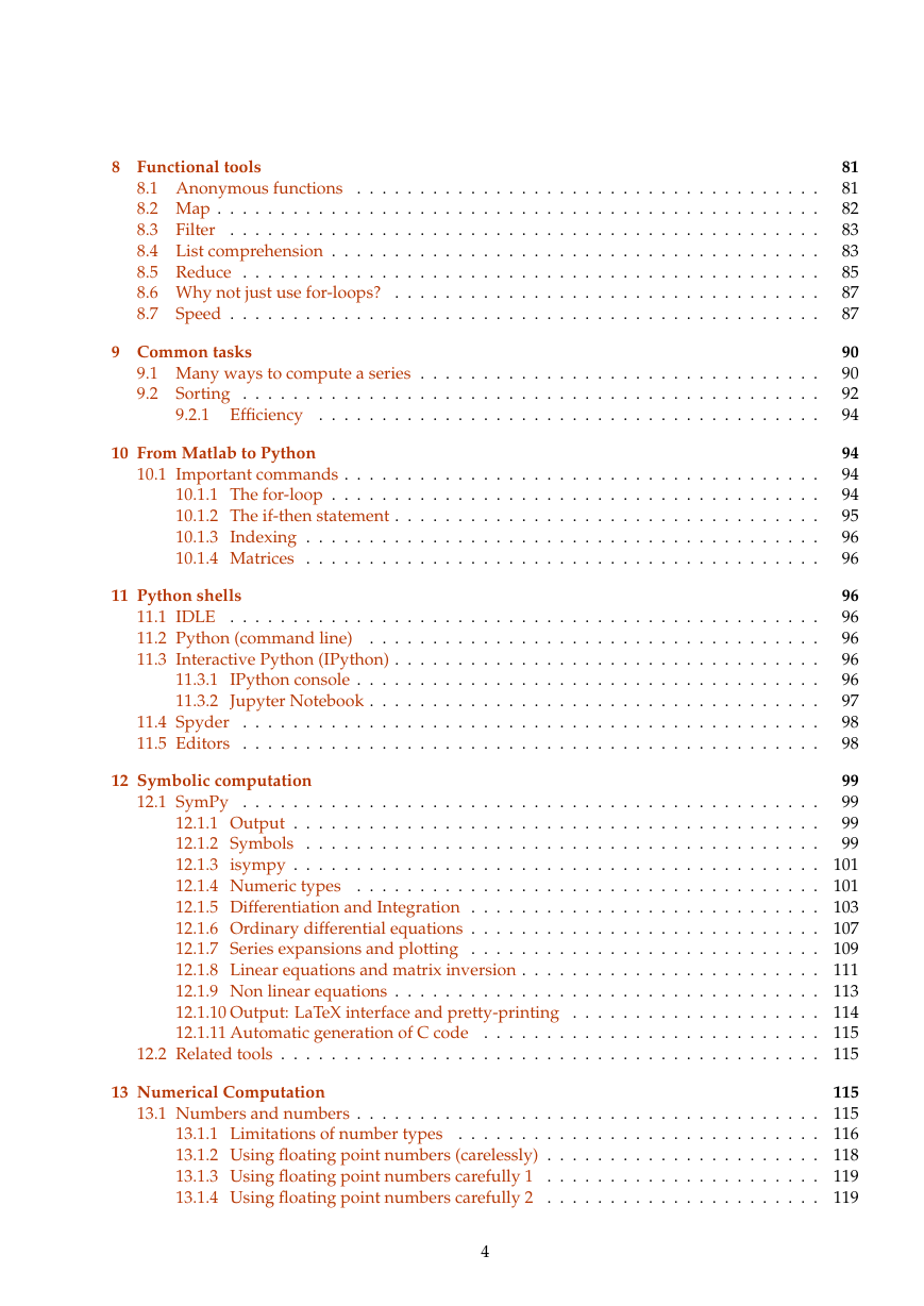
8 Functional tools . . . . . . . . . . . . . . . . . . . . . . . . . . . . . . . . . . . . . . . . . . . . . . . . . . 8.1 Anonymous functions . . . . . . . . . . . . . . . . . . . . . . . . . . . . . . . . . . . 8.2 Map . . . . . . . . . . . . . . . . . . . . . . . . . . . . . . . . . . . . 8.3 Filter . . . . . . . . . . . . . . . . . . . . . . . . . . . . . . . . . . . 8.4 List comprehension . . . . . . . . . . . . . . . . . . . . . . . . . . . . . . . . . . 8.5 Reduce . . . 8.6 Why not just use for-loops? . . . . . . . . . . . . . . . . . . . . . . . . . . . . . . . . . 8.7 . . . . . . . . . . . . . . . . . . . . . . . . . . . . . . . . . . Speed . . . . . . . . . . . . . . . . . . . . . . . . . . . . . . . 9 Common tasks 9.1 Many ways to compute a series . . . . . . . . . . . . . . . . . . . . . . . . . . . . . . . . 9.2 . . . . . . . . . . . . . . . . . . . . . . . . . . . . . . . . . . . . . . . . . . . . . . . . . . . . . . . . . . . . . . . . . Sorting . . 9.2.1 Efficiency . . . . . . . . . . . . . . . . 10 From Matlab to Python 10.1 Important commands . . . . . . . . . . . . . . . . . . . . . . . . . . . . . . . . . . . . 10.1.1 The for-loop . . . . . . . . . . . . . . . . . . . . . . . . . . . . . . . . . . . 10.1.2 The if-then statement . . . . . . . . . . . . . . . . . . . . . . . . . . . . . . . . . . . . . . . . . . . . . . . . . . . . . . . . . . . . . . . . . . 10.1.3 Indexing . 10.1.4 Matrices . . . . . . . . . . . . . . . . . . . . . . . . . . . . . . . . . . . . . . . . . . . . . . . . . . . . . . . . . . . 11 Python shells . . . . . . . . . . . . . . . . . . . . . . . . . . . . . . . . . 11.1 IDLE . . 11.2 Python (command line) . . . . . . . . . . . . . . . . . . . . . . . . . . . . . . . . . 11.3 Interactive Python (IPython) . . . . . . . . . . . . . . . . . . . . . . . . . . . . . . . . . . . . . . . . . . . . . . . . . . . . . . . . . . . . . . . . . . . . . . . . . . . . . . . . . . . . . . . . . . . . . . . . . . . . . . . . . . . . . . . . . . . . . . . . . . . . . . . . . . . . . . . . . . . . . . . . . . . . . . . . . . . . . . . . . . . . . . . 11.3.1 IPython console . . 11.3.2 Jupyter Notebook . . . 11.4 Spyder . 11.5 Editors . . . . . . . . . . . . . . . . . . . . . . . . . . . . . . . . . . . . . . . . . . . . . . 12.1 SymPy . 12 Symbolic computation . . . . . . . . . . . . . . . . . . . . . . . . . . . . . . . . . . . . . . . . . . . . . . . . . . . . . . . . . . . . . . . . . . . . . . . . 12.1.1 Output . . . . . . . . . . . . . . . . . . . . . . . . . . . . . . . . . . . . . 12.1.2 Symbols . . . . . . . . . . . . . . . . . . . . . . . . . . . . . . . . . . . 12.1.3 isympy . . . 12.1.4 Numeric types . . . . . . . . . . . . . . . . . . . . . . . . . . . . . . . . . . 12.1.5 Differentiation and Integration . . . . . . . . . . . . . . . . . . . . . . . . . . . 12.1.6 Ordinary differential equations . . . . . . . . . . . . . . . . . . . . . . . . . . . 12.1.7 Series expansions and plotting . . . . . . . . . . . . . . . . . . . . . . . . . . . 12.1.8 Linear equations and matrix inversion . . . . . . . . . . . . . . . . . . . . . . . 12.1.9 Non linear equations . . . . . . . . . . . . . . . . . . . . . . . . . . . . . . . . . 12.1.10 Output: LaTeX interface and pretty-printing . . . . . . . . . . . . . . . . . . . 12.1.11 Automatic generation of C code . . . . . . . . . . . . . . . . . . . . . . . . . . . . . . . . . . . . . . . . . . . . . . . . . . . . . . . . . . 12.2 Related tools . . . . . . . . . . 13 Numerical Computation . 13.1 Numbers and numbers . . . . . . . . . . . . . . . . . . . . . . . . . . . . . . . . . . . 13.1.1 Limitations of number types . . . . . . . . . . . . . . . . . . . . . . . . . . . . 13.1.2 Using floating point numbers (carelessly) . . . . . . . . . . . . . . . . . . . . . 13.1.3 Using floating point numbers carefully 1 . . . . . . . . . . . . . . . . . . . . . 13.1.4 Using floating point numbers carefully 2 . . . . . . . . . . . . . . . . . . . . . 4 81 81 82 83 83 85 87 87 90 90 92 94 94 94 94 95 96 96 96 96 96 96 96 97 98 98 . . . . . . . . . . . . . . . . . . . . . . 99 99 . 99 . . 99 . 101 . 101 . 103 . 107 . 109 . 111 . 113 . 114 . 115 . 115 115 . 115 . 116 . 118 . 119 . 119
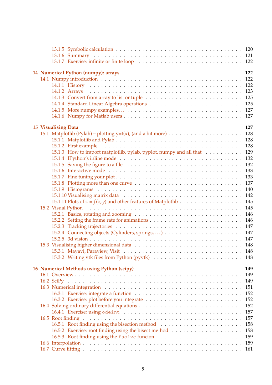
13.1.5 Symbolic calculation . . . . . . . . . . . . . . . . . . . . . . . . . . . . . . . . . . 13.1.6 Summary . . . . . . . . . . . . . . . . . . . . . . . . . . . . . . . . . . 13.1.7 Exercise: infinite or finite loop . . . . . . . . . . . . . . . . . . . . . . . . . . . . . . . 14 Numerical Python (numpy): arrays . . . . . . . . . . . 14.1 Numpy introduction . . . . . . . . . . . . . . . . . . . . . . . . . . . . . . . . . . . . . . . . . . . . . . . . . . . . . . . . . . . . . . . . . . . . . . 14.1.1 History . 14.1.2 Arrays . . . . . . . . . . . . . . . . . . . . . . . . . . . . . . . . . . . 14.1.3 Convert from array to list or tuple . . . . . . . . . . . . . . . . . . . . . . . . . 14.1.4 Standard Linear Algebra operations . . . . . . . . . . . . . . . . . . . . . . . . 14.1.5 More numpy examples. . . . . . . . . . . . . . . . . . . . . . . . . . . . . . . . . 14.1.6 Numpy for Matlab users . . . . . . . . . . . . . . . . . . . . . . . . . . . . . . . . . 15 Visualising Data . . . . . . . . . . . . . . . . . . . . . . . . . . . . . . . . . . . . . . . . . . . . . . . . . . . . . . . . . . . . . . . . 15.1 Matplotlib (Pylab) – plotting y=f(x), (and a bit more) . . . . . . . . . . . . . . . . . . . 15.1.1 Matplotlib and Pylab . . . . . . . . . . . . . . . . . . . . . . . . . . . . . . . . . 15.1.2 First example . . . . . . . . . . . . . . . . . . . . . . . . . . . . . . . . . . . 15.1.3 How to import matplotlib, pylab, pyplot, numpy and all that . . . . . . . . . 15.1.4 IPython’s inline mode . . . . . . . . . . . . . . . . . . . . . . . . . . . . . . . . . 15.1.5 Saving the figure to a file 15.1.6 Interactive mode . . . . . . . . . . . . . . . . . . . . . . . . . . . . . . . . . . 15.1.7 Fine tuning your plot . . 15.1.8 Plotting more than one curve . . . . . . . . . . . . . . . . . . . . . . . . . . . 15.1.9 Histograms . . . . . . . . . . . . . . . . . . . . . . . . . . . . . . . . . . . 15.1.10 Visualising matrix data . . . . . . . . . . . . . . . . . . . . . . . . . . . . . . . 15.1.11 Plots of z = f (x, y) and other features of Matplotlib . . . . . . . . . . . . . . . . . . . . . . . . . . . . . . . . . . . . . . . . . . . . . . . . 15.2.1 Basics, rotating and zooming . . . . . . . . . . . . . . . . . . . . . . . . . . . . 15.2.2 Setting the frame rate for animations . . . . . . . . . . . . . . . . . . . . . . . . 15.2.3 Tracking trajectories . . . . . . . . . . . . . . . . . . . . . . . . . . . . . . . . . 15.2.4 Connecting objects (Cylinders, springs, . . . ) . . . . . . . . . . . . . . . . . . . . 15.2.5 3d vision . . 15.3 Visualising higher dimensional data . . . . . . . . . . . . . . . . . . . . . . . . . . . . . . . . . . . . . . . . . . . . . . . . . . . . 15.3.1 Mayavi, Paraview, Visit 15.3.2 Writing vtk files from Python (pyvtk) . . . . . . . . . . . . . . . . . . . . . . . . . . . . . . . . . . . . . . . . . . . . . . . . . . . . . . . . . . . . . . 15.2 Visual Python . . . . . . . . . . . . . . . . . . 16 Numerical Methods using Python (scipy) . . . . . . . . . . . . . . . . . . 16.4 Solving ordinary differential equations . . . . . . . . . . . . . . . . . . . . . . . . . . . 16.1 Overview . 16.2 SciPy . . . 16.3 Numerical integration . . . . . . . . . . . . . . . . . . . . . . . . . . . . . . . . . . . . . . . . . . . . . . . . . . . . . . . . . . . . . . . . . . . . . . . . . . . . . . . . . . . . . . . . . . . . . . . . . . . . . . . 16.3.1 Exercise: integrate a function . . . . . . . . . . . . . . . . . . . . . . . . . . . . 16.3.2 Exercise: plot before you integrate . . . . . . . . . . . . . . . . . . . . . . . . . . 16.4.1 Exercise: using odeint . . . . . . . . . . . . . . . . . . . . . . . . . . . . . . . . . . . . . . . . . . . . . . . . . . . . . . . . . . . . . . . . . 16.5.1 Root finding using the bisection method . . . . . . . . . . . . . . . . . . . . . 16.5.2 Exercise: root finding using the bisect method . . . . . . . . . . . . . . . . . . 16.5.3 Root finding using the fsolve funcion . . . . . . . . . . . . . . . . . . . . . . . . . . . . . . . . . . . . . . . . . . . . . . . . . . . . . . . . . . . . . . . . . . . . . . . . . . . . . . . . . . . . . . . . . 16.6 Interpolation . 16.7 Curve fitting . 16.5 Root finding . . . . . . . . . . . . . . . . . . . . . . . 5 . 120 . 121 . 122 122 . 122 . 122 . 123 . 125 . 125 . 127 . 127 127 . 128 . 128 . 128 . 129 . 132 . 132 . 133 . 133 . 137 . 140 . 142 . 145 . 145 . 146 . 146 . 147 . 147 . 147 . 148 . 148 . 148 149 . 149 . 149 . 151 . 152 . 152 . 152 . 157 . 157 . 158 . 158 . 159 . 159 . 161
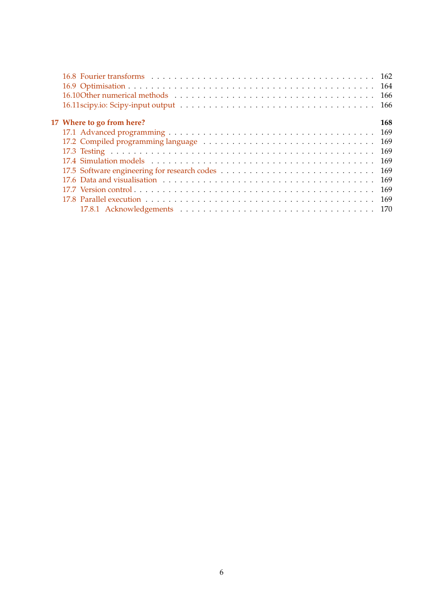
. . . . . . . . . . . . . . . . . . . . . . . . . . . . . . . . . 16.8 Fourier transforms 16.9 Optimisation . . . . . . . . . . . . . . . . . . . . . . . . . . . . . . . . . . . . 16.10Other numerical methods . . . . . . . . . . . . . . . . . . . . . . . . . . . . . . . . . . . . . . . . . . . . . . . . . . . . . . . . . . . . . . . . . . . 16.11scipy.io: Scipy-input output . . . . . . . . . . . 17 Where to go from here? . . . . . . . . 17.1 Advanced programming . . . . . . . . . . . . . . . . . . . . . . . . . . . . . . . . . 17.2 Compiled programming language . . . . . . . . . . . . . . . . . . . . . . . . . . . . . . 17.3 Testing . . . . . . . . . . . . . . . . . . . . . . . . . . . . . . . . . . 17.4 Simulation models . . . . . . . . . . . . . . . . . . . . . . . . . . . . . . . . . . 17.5 Software engineering for research codes . . . . . . . . . . . . . . . . . . . . . . . . . . . 17.6 Data and visualisation . . . . . . . . . . . . . . . . . . . . . . . . . . . . . . . . . . . . . . . . . . . . . . . . . . . . . . . . . . . . . . . . . . . . . 17.7 Version control . . 17.8 Parallel execution . . . . . . . . . . . . . . . . . . . . . . . . . . . . . . . . . . . . . . . . . . . . . . . . . . . . . . . . . . . . . . . . . . . . . . . . 17.8.1 Acknowledgements . . . . . . . . . . . . . . 162 . 164 . 166 . 166 168 . 169 . 169 . 169 . 169 . 169 . 169 . 169 . 169 . 170 6
1 Introduction This text summarises a number of core ideas relevant to Computational Engineering and Scientific Computing using Python. The emphasis is on introducing some basic Python (programming) con- cepts that are relevant for numerical algorithms. The later chapters touch upon numerical libraries such as numpy and scipy each of which deserves much more space than provided here. We aim to enable the reader to learn independently how to use other functionality of these libraries using the available documentation (online and through the packages itself). 1.1 Computational Modelling 1.1.1 Introduction Increasingly, processes and systems are researched or developed through computer simulations: new aircraft prototypes such as for the recent A380 are first designed and tested virtually through com- puter simulations. With the ever increasing computational power available through supercomputers, clusters of computers and even desktop and laptop machines, this trend is likely to continue. Computer simulations are routinely used in fundamental research to help understand experi- mental measurements, and to replace – for example – growth and fabrication of expensive samples/- experiments where possible. In an industrial context, product and device design can often be done much more cost effectively if carried out virtually through simulation rather than through build- ing and testing prototypes. This is in particular so in areas where samples are expensive such as nanoscience (where it is expensive to create small things) and aerospace industry (where it is expen- sive to build large things). There are also situations where certain experiments can only be carried out virtually (ranging from astrophysics to study of effects of large scale nuclear or chemical ac- cidents). Computational modelling, including use of computational tools to post-process, analyse and visualise data, has been used in engineering, physics and chemistry for many decades but is becoming more important due to the cheap availability of computational resources. Computational Modelling is also starting to play a more important role in studies of biological systems, the economy, archeology, medicine, health care, and many other domains. 1.1.2 Computational Modelling To study a process with a computer simulation we distinguish two steps: the first one is to develop a model of the real system. When studying the motion of a small object, such as a penny, say, under the influence of gravity, we may be able to ignore friction of air: our model — which might only consider the gravitational force and the penny’s inertia, i.e. a(t) = F/m = −9.81m/s2 — is an approximation of the real system. The model will normally allow us to express the behaviour of the system (in some approximated form) through mathematical equations, which often involve ordinary differential equations (ODEs) or partial differential equatons (PDEs). In the natural sciences such as physics, chemistry and related engineering, it is often not so diffi- cult to find a suitable model, although the resulting equations tend to be very difficult to solve, and can in most cases not be solved analytically at all. On the other hand, in subjects that are not as well described through a mathematical framework and depend on behaviour of objects whose actions are impossible to predict deterministically (such as humans), it is much more difficult to find a good model to describe reality. As a rule of thumb, in these disciplines the resulting equations are easier to solve, but they are harder to find and the validity of a model needs to be questioned much more. Typical examples are attempts to simulate the economy, the use of global resources, the behaviour of a panicking crowd, etc. So far, we have just discussed the development of models to describe reality, and using these models does not necessarily involve any computers or numerical work at all. In fact, if a model’s 7
equation can be solved analytically, then one should do this and write down the solution to the equation. In practice, hardly any model equations of systems of interest can be solved analytically, and this is where the computer comes in: using numerical methods, we can at least study the model for a particular set of boundary conditions. For the example considered above, we may not be able to easily see from a numerical solution that the penny’s velocity under the influence of gravity will change linearly with time (which we can read easily from the analytical solution that is available for this simple system: v(t) = t · 9.81m/s2 + v0)). The numerical solution that can be computed using a computer would consist of data that shows how the velocity changes over time for a particular initial velocity v0 (v0 is a boundary condition here). The computer program would report a long lists of two numbers keeping the (i) value of time ti for which a particular (ii) value of the velocity vi has been computed. By plotting all vi against ti, or by fitting a curve through the data, we may be able to understand the trend from the data (which we can just see from the analytical solution of course). It is clearly desirable to find an analytical solutions wherever possible but the number of prob- lems where this is possible is small. Usually, the obtaining numerical result of a computer simulation is very useful (despite the shortcomings of the numerical results in comparison to an analytical ex- pression) because it is the only possible way to study the system at all. The name computational modelling derives from the two steps: (i) modelling, i.e. finding a model de- scription of a real system, and (ii) solving the resulting model equations using computational methods because this is the only way the equations can be solved at all. 1.1.3 Programming to support computational modelling A large number of packages exist that provide computational modelling capabilities. If these satisfy the research or design needs, and any data processing and visualisation is appropriately supported through existing tools, one can carry out computational modelling studies without any deeper pro- gramming knowledge. In a research environment – both in academia and research on new products/ideas/. . . in in- dustry – one often reaches a point where existing packages will not be able to perform a required simulation task, or where more can be learned from analysing existing data in news ways etc. At that point, programming skills are required. It is also generally useful to have a broad under- standing of the building blocks of software and basic ideas of software engineering as we use more and more devices that are software-controlled. It is often forgotten that there is nothing the computer can do that we as humans cannot do. The computer can do it much faster, though, and also with making far fewer mistakes. There is thus no magic in computations a computer carries out: they could have been done by humans, and – in fact – were for many years (see for example Wikipedia entry on Human Computer). Understanding how to build a computer simulation comes roughly down to: (i) finding the model (often this means finding the right equations), (ii) knowing how to solve these equations numerically, (ii) to implement the methods to compute these solutions (this is the programming bit). 1.2 Why Python for scientific computing? The design focus on the Python language is on productivity and code readability, for example through: • Interactive python console • Very clear, readable syntax through whitespace indentation • Strong introspection capabilities 8
分享到:
收藏