加权最小二乘法，近似完美的最小最大拟合.pdf-资料库

Applied Mathematics, 2017, 8, 645-654 http://www.scirp.org/journal/am ISSN Online: 2152-7393 ISSN Print: 2152-7385 Weighted Least-Squares for a Nearly Perfect Min-Max Fit Isaac Fried, Ye Feng Department of Mathematics, Boston University, Boston, MA, USA How to cite this paper: Fried, I. and Feng, Y. (2017) Weighted Least-Squares for a Nearly Perfect Min-Max Fit. Applied Ma- thematics, 8, 645-654. https://doi.org/10.4236/am.2017.85051 Received: February 28, 2017 Accepted: May 19, 2017 Published: May 22, 2017 Copyright © 2017 by authors and Scientific Research Publishing Inc. This work is licensed under the Creative Commons Attribution International License (CC BY 4.0). http://creativecommons.org/licenses/by/4.0/ Abstract In this note, we experimentally demonstrate, on a variety of analytic and nonanalytic functions, the novel observation that if the least squares poly- nomial approximation is repeated as weight in a second, now weighted, least squares approximation, then this new, second, approximation is nearly perfect in the uniform sense, barely needing any further, say, Remez correction. Keywords Least Squares-Approximation of Functions, Weighted Approximations, Nearly Perfect Uniform Fits Open Access 1. Introduction Finding the min-max, or best L∞ , polynomial approximation to a function, in some standard interval, is of the greatest interest in numerical analysis [1] [2]. For a polynomial function the least error distribution is a Chebyshev polynomial [3] [4] [5]. The usual procedure [6] [7] to find the best L∞ approximation to a general 2L sense, easily ob- function is to start with a good approximation, say in the tained by the minimization of a quadratic functional for the coefficients, then iteratively improving this initial approximation by a Remez-like correction pro- cedure [8] [9] that strives to produce an error distribution that oscillates with a constant amplitude in the interval of interest. In this note, we bring ample and varied computational evidence in support of the novel, worthy of notice, empirical numerical observation that taking the er- 2L , best polynomial fit to a function, squared, ror distribution of a least squares, as weight in a second, weighted, least squares approximation, results in an error distribution that is remarkably close to the best L∞ , or uniform, approximation. DOI: 10.4236/am.2017.85051 May 22, 2017

I. Fried, Y. Feng 2. Fixing Ideas; The Best Quadratic in [−1, 1] The monic Chebyshev polynomial ( ) T x 2 = − 1 x x 2 1 , 1 2 − ≤ ≤ (1) is the solution of the min-max problem ( ) e x ( ) e x , min max a x = 2 x − a − ≤ ≤ (2) , 1 1. x x This min-max solution, the least function in the L∞ sense, is a polynomial that has two distinct roots, and oscillates with a constant amplitude in ( ( ) e e 1 . = is such a po- − ≤ ≤ 1, 1 p x e≤ lynomial, and + 1 2 2e would intersect at two points, which is 1e and in the interval, for otherwise p x p absurd; is either an identity, or has but the one + + 1 0 ) p a − solution . 1 1 Indeed, say is another quadratic polynomial, then ) 1 − = − 2 e x = 2 ( ) e 0 p + 0 a x = 1 a − 0 a + 0 = − x ) ( + p 0 x x a x 1 a 0 e 1 e 1 = + + x ( 2 2 2 Thus, the monic Chebyshev polynomial of degree n is the least, uniform, or nx by a polynomial of degree pointwise, error distribution in approximating 1n − . To obtain a least squares, a best nimize ( ) I a 2L , approximation to 2T x we first mi- ( ) ( I a 2 1 2 ′ 1 − ) ) x a = − = ( x I a d , ) ∫ 1 3 0.3333 I p , under the weight ( ( ) 1 3 = ( = ) ) ( ( x I p d , − . p ) x 2 2 2 to have the value a = Minimizing next ( I p ) = ( 2 x − 1 1 − ∫ p = now with respect to p, we obtain closer to the optimal value of one half. ( 2 x − a ) d x = 0 (3) 1 1 − ∫ a 2 ′ x ∫ − ( 11 21 0.5238 = x 1 − 1 2 1 3 , )2 − a = )( p x 2 − 1 3 d x = 0 (4) 2 ) , which is surprisingly much We may replace the difficult L∞ measure by the computationally easier mL a δ measure with an even + 0 be an improved one. Minimization cum linearization produces the equation 1m  . Let a0 be a good approximation, and a 1 = 1 1 − ( 2 x − a 0 n ) d x n − ∫ δ 1 1 − ( 2 x − a 0 n − ) 1 d x = 0 (5) where ∫ n  is odd. a = 0 a = 1 Starting with 17 , the value 1 n = 11 21 0.5238 = , as compared with the optimal 0.495 , we obtain from the above equation, for a = 0.5 . 3. Optimal Cubic in [−1, 1] Seeking to reproduce the optimal monic Chebyshev polynomial of degree three ( ) T x 3 = 3 x − 3 , 1 x 4 − ≤ ≤ (6) 1 x we start by minimizing ∫ ( I a 1 = ) )1 ( I a ( 1 − x 3 1 − a x 1 2 ) ( x I a d , 1 ′ ) = 646 ( x x 3 − a x 1 ) x d = 0 (7) 1 1 − ∫

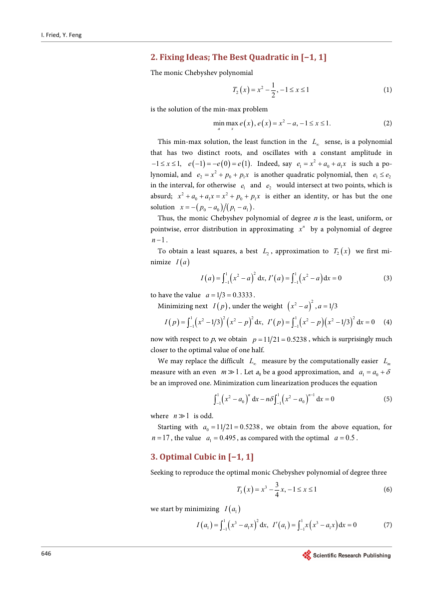
I. Fried, Y. Feng and have a = 1 3 5 = 0.6 . Then we return to minimize the weighted ) ( x ) ( 2 a x 1 ( I p 1 ( ′ I p 1 ( x ( x x ) ) a x 1 1 − 1 = − = − 2 1 3 3 ∫ ∫ 3 1 − 2 )1 ) p x 1 p x 1 − − 3 x ( I p with respect to 1p x d , ) d x (8) = 0 and obtain = value of 0.75. See Figure 1. p = 1 195 253 0.770751 , which is considerably closer to the optimal We are ready now for a Remez-like correction to bring the error function closer occurs at m = 0.50687. We , by which x and request that ( ) e x 3 x − x 0.770751 ( e m e ( )1 = a x 1 to optimal. The minimum of = write a new tentative we have ( ) e x − − = ) 3 a 1 = 1 + 1 + 3 m m = 0.750047 (9) as compared with the Chebyshev optimal value of a = 1 3 4 = 0.75 . 4. 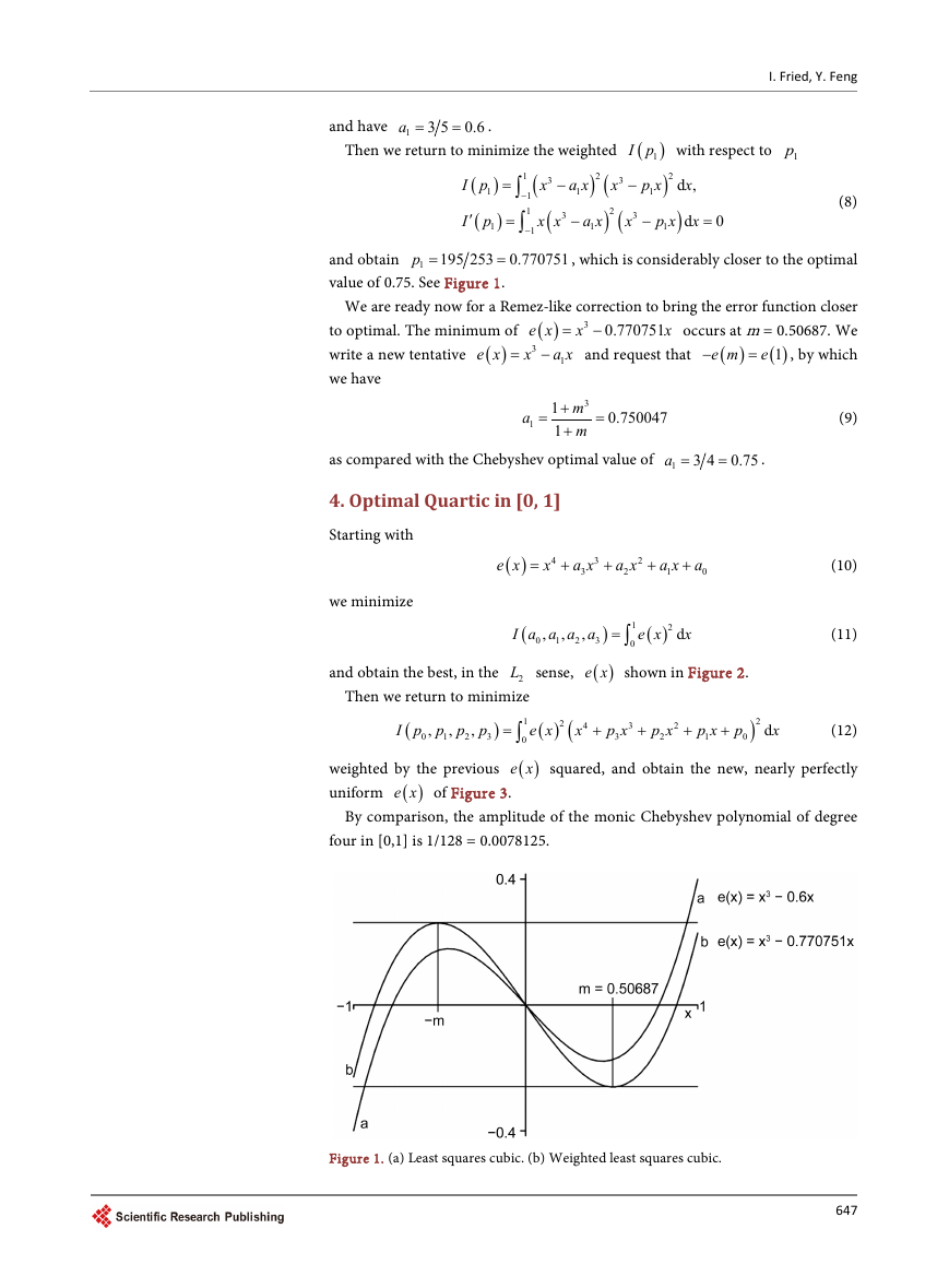Optimal Quartic in [0, 1] Starting with ( ) e x = 4 x + 3 a x 3 + 2 a x 2 + a x a 1 0 + (10) we minimize and obtain the best, in the 2L sense, ( I a a a a , 3 , , 0 1 2 1 0 2 x d = ∫ ( ) e x ) ( ) e x shown in Figure 2. 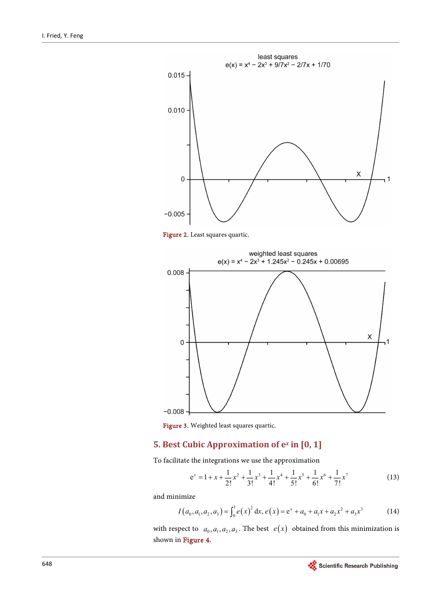(11) Then we return to minimize 1 ∫ ( ) e x squared, and obtain the new, nearly perfectly ( I p p p p 3 (12) ( ) ( e x p x 2 p x 3 p x 1 )2 x d p 0 = + + + + x ) , , , 2 4 3 2 0 0 1 2 weighted by the previous uniform ( ) e x of Figure 3. By comparison, the amplitude of the monic Chebyshev polynomial of degree four in [0,1] is 1/128 = 0.0078125. Figure 1. (a) Least squares cubic. (b) Weighted least squares cubic. 647

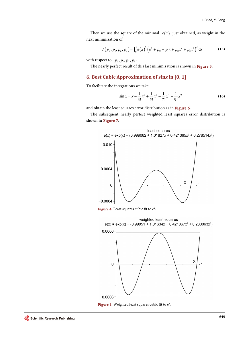
I. Fried, Y. Feng 648 + 1 7! 7 x (13) Figure 2. Least squares quartic. Figure 3. Weighted least squares quartic. 5. Best Cubic Approximation of ex in [0, 1] To facilitate the integrations we use the approximation 1 6! = + + 1 4! 1 2! 1 5! 1 3! + + + + 1 x x x x x x e 2 3 4 5 x 6 and minimize , ( I a a a a , 3 , 0 1 2 ) = 1 0 ∫ , 2 ( ) e x ( ) x e x d , + + + = a 0 a x a x 1 2 ex ( ) e x obtained from this minimization is (14) a x 3 + 2 3 a a a a . The best with respect to , 0 shown in Figure 4. , 1 2 3

Then we use the square of the minimal ( ) e x just obtained, as weight in the next minimization of I. Fried, Y. Feng ( I p p p p 3 , , , 0 1 2 ) = 1 0 ∫ ( ) ( e x 2 x e + p 0 + p x 1 + 2 p x 2 + 3 p x 3 )2 x d (15) with respect to p p p p . 0 3 , , , 1 2 The nearly perfect result of this last minimization is shown in Figure 5. 6. Best Cubic Approximation of sinx in [0, 1] To facilitate the integrations we take sin x = − x 1 3! 3 x + 1 5! 5 x − 1 7! 7 x + 1 9! 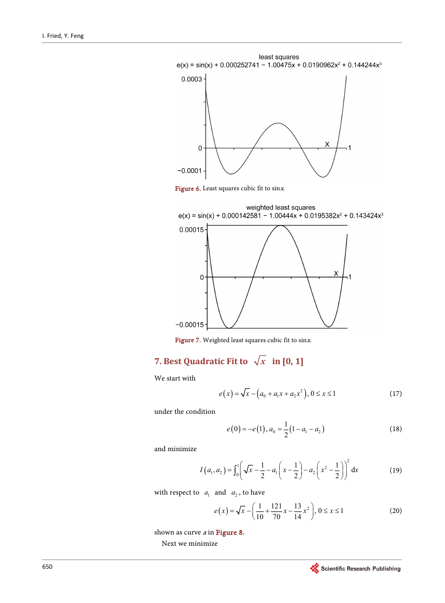9 x (16) and obtain the least squares error distribution as in Figure 6. The subsequent nearly perfect weighted least squares error distribution is shown in Figure 7. Figure 4. Least squares cubic fit to ex. Figure 5. Weighted least squares cubic fit to ex. 649

I. Fried, Y. Feng Figure 6. Least squares cubic fit to sinx. Figure 7. Weighted least squares cubic fit to sinx. 7. Best Quadratic Fit to x in [0, 1] We start with under the condition ( ) e x = x − ( a 0 + a x a x 1 2 + )2 , 0 ≤ ≤ (17) 1 x e ( ) 0 = − e ( ) 1 , a 0 = 1 2 ( 1 − a 1 − a 2 ) (18) and minimize ( I a a , 2 1 ) = 1 0 ∫    x − − 1 2  a x  1  − 1 2    − a 2    2 x − 2 1 2       d x (19) with respect to 1a and ( ) e x 2a , to have 1 10    − x = + 121 70 x − 13 14 2 x    , 0 ≤ ≤ x 1 (20) 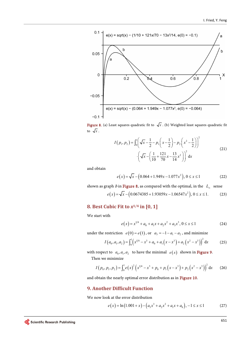shown as curve a in Figure 8. Next we minimize 650

I. Fried, Y. Feng Figure 8. (a) Least squares quadratic fit to to x . x . (b) Weighted least squares quadratic fit ( I p p 2 , 1 ) = 1 ∫ 0       ⋅ − x − − 1 2 x −    1 10  p x  1  121 70 + 1 2 −    13 14 p 2    2 x − 2 1 2       2 x 2       d x (21) x − and obtain ( ) e x = x − ( 0.064 1.949 + x − 1.077 x )2 , 0 ≤ ≤ (22) 1 x shown as graph b in Figure 8, as compared with the optimal, in the L∞ sense ( ) e x = x − ( 0.0674385 1.93059 + x − 1.06547 x , 0 ≤ ≤ (23) 1. x )2 8. 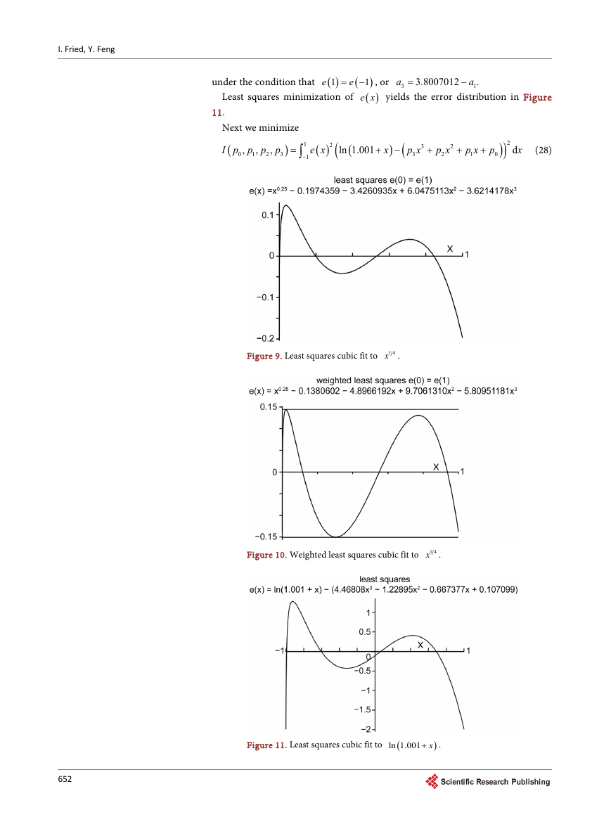Best Cubic Fit to x1/4 in [0, 1] We start with + a 0 ( ) 1 ( ) e x = 1 4 x + a x a x 1 2 + 2 + 3 a x 3 , 0 ≤ ≤ (24) 1 x e a 3 e= , or ( ) 0 ( 1 ∫ 1 = − − ( a x 1 a a a to have the minimal 0 1 4 x a 0 = − + + x , 3 0 2 − 3 x a 1 a 2 , and minimize ( a x 2 − ) ( ) e x shown in Figure 9. )2 + − d ) x x 2 3 (25) under the restriction ) ( I a a a , 2 , 0 1 with respect to , 1 Then we minimize 1 ∫ ( I p p p 2 = ) , , 1 0 0 2 ( ) e x ( 1 4 x − 3 x + p 0 + ( p x 1 − 3 x ) + ( p x 2 2 − 3 x ) )2 d x (26) and obtain the nearly optimal error distribution as in Figure 10. 9. Another Difficult Function We now look at the error distribution 3 a x 3 ln 1.001 ( ) e x = + − x ( ) ( + 2 a x 2 + a x a 1 0 + ) , 1 − ≤ ≤ (27) 1 x 651

I. Fried, Y. Feng under the condition that ( e= Least squares minimization of ( ) 1 e 11. a 3 ) − , or 1 ( ) e x yields the error distribution in Figure 3.8007012 a 1 = − . Next we minimize ( ∫ I p p p p 3 = ) , , , 0 1 2 1 1 − 2 ( ) e x ( ln 1.001 ( + ) − ( x 3 p x 3 + 2 p x 2 + p x 1 + p 0 ) )2 x d (28) Figure 9. Least squares cubic fit to 1 4x . Figure 10. Weighted least squares cubic fit to 1 4x . Figure 11. Least squares cubic fit to ln 1.001 x+ ( ) . 652

资料库

加权最小二乘法，近似完美的最小最大拟合.pdf

相关推荐

开发技术

热门标签

最新资料