COOLCAT: An entropy-based algorithm for categorical clustering
Daniel Barbara
Julia Couto
Yi Li
George Mason University
Information and Software Engineering Department
Fairfax, VA �����
Phone: ���- �����, Fax=���- �����
{dbarbara,jics,yli�}@gmu.edu
October �, ����
Abstract
Clustering of categorical attributes is a dicult problem that has not received as much at-
tention as its numerical counterpart. In this paper we explore the connection between clustering
and entropy: clusters of similar points have lower entropy than those of dissimilar ones. We use
this connection to design a heuristic algorithm, COOLCAT, which is capable of eciently cluster
large data sets of records with categorical attributes. In contrast with other categorical clustering
algorithms published in the past, COOLCAT’s clustering results are very stable for dierent sam-
ple sizes and parameter settings. Also, the criteria for clustering is a very intuitive one, since it is
deeply rooted on the well-known notion of entropy. We demonstrate the eciency and scalability
of COOLCAT by a series of experiments on real and synthetic data sets.
�
Introduction
Clustering is a widely used technique in which data points are partitioned into groups, in such a
way that points in the same group, or cluster, are more similar among themselves than to those in
other clusters. Clustering of categorical attributes (i.e., attributes whose domain is not numeric) is
a dicult, yet important task: many elds, from statistics to psychology deal with categorical data.
In spite of its importance, the task of categorical clustering has received scant attention in the KDD
community as of late, with only a handful of publications addressing the problem ([��, ��, ��]).
Much of the published algorithms to cluster categorical data rely on the usage of a distance
metric that captures the separation between two vectors of categorical attributes, such as the Jaccard
coecient [��]. In this paper, we present COOLCAT (the name comes from the fact that we reduce
the entropy of the clusters, thereby \cooling" them), a novel method which uses the notion of entropy
to group records. We argue that a classical notion such as entropy is a more natural and intuitive
way of relating records, and more importantly does not rely in arbitrary distance metrics.
This paper is set up as follows. Section � oers the background and relationship between entropy
and clustering, and formulates the problem. Section � reviews the related work. Section � describes
COOLCAT, our algorithm. Section � presents the experimental evidence that demonstrates the
advantages of COOLCAT. Finally, Section � presents conclusions and future work.
This work has been supported by NSF grant IIS- ������
�
�
� Background and problem formulation
In this section, we present the background of entropy and clustering and formulate the problem.
�.� Entropy and Clustering
Entropy is the measure of information and uncertainty of a random variable [��]. Formally, if X is
a random variable, S(X) the set of values that X can take, and p(x) the probability function of X,
the entropy E(X) is dened as shown in Equation �.
E(X) = X
p(x)log(p(x))
x � S(X)
(�)
The entropy of a multivariate vector ^x = fX�; ; Xng can be computed as shown in Equation
�.
E(^x) = X
X
p(x�; ; xn)logp(x�; ; xn)
(�)
x� � S(X�)
xn � S(Xn)
Entropy is sometimes referred to as a measure of the amount of "disorder" in a system. A room
with socks strewn all over the oor has more entropy than a room in which socks are paired up,
neatly folded, and placed in one side of your sock and underwear drawer.
�.� Problem formulation
j ; ; pd
The problem we are trying to solve can be formulated as follows. Given a data set D of N
points ^p�; ; ^pN , where each point is a multidimensional vector of d categorical attributes, i.e.,
^pj = (p�
j ), and given an integer k, we would like to separate the points into k groups
C�; ; Ck, or clusters, in such a way that we minimize the entropy of the whole arrangement. Un-
fortunately, this problem is NP-Complete, and moreover, dicult to approximate [��]. In fact, the
problem is NP-Complete for any distance function d(x; y), dened over pairs of points x; y, such
that the function maps pairs of points to real numbers (and hence, our entropic function qualies),
therefore we need to resort to heuristics to solve it.
We rst have to resolve the issue of what we mean by the \whole entropy of the system." In
other words, we have to make our objective function clear. We aim to minimize the expected entropy,
whose expression is shown in Equation �, where E(P (C�)); ; E(P (Ck)), represent the entropies of
each cluster, P (Ci) denotes the points assigned to cluster Ci, P (Ci) D, with the property that
P (Ci) \ P (Cj) = ;, for all i; j = �; ::; k i �= j. The symbol C = fC�; ; Ckg represents the
clustering.
E( C) = X
(
k
jP (Ck)j
jDj
(E(P (Ck))))
(�)
This function, as we will see later, allows us to implement an incremental algorithm that can
eectively deal with large datasets, since we do not need to look at the entire set of points to decide
about the entropy of an arrangement. Rather, we will be able to decide for each point, how it would
aect the entropy of each of the existing clusters if placed in each one of them.
The solution we propose in this paper (and present in Section �) is a heuristic based in nding
a set of initial clusters (using the entropic criteria), and then incrementally (greedily) add points to
the clusters according to a criteria that minimizes Equation �.
�
�
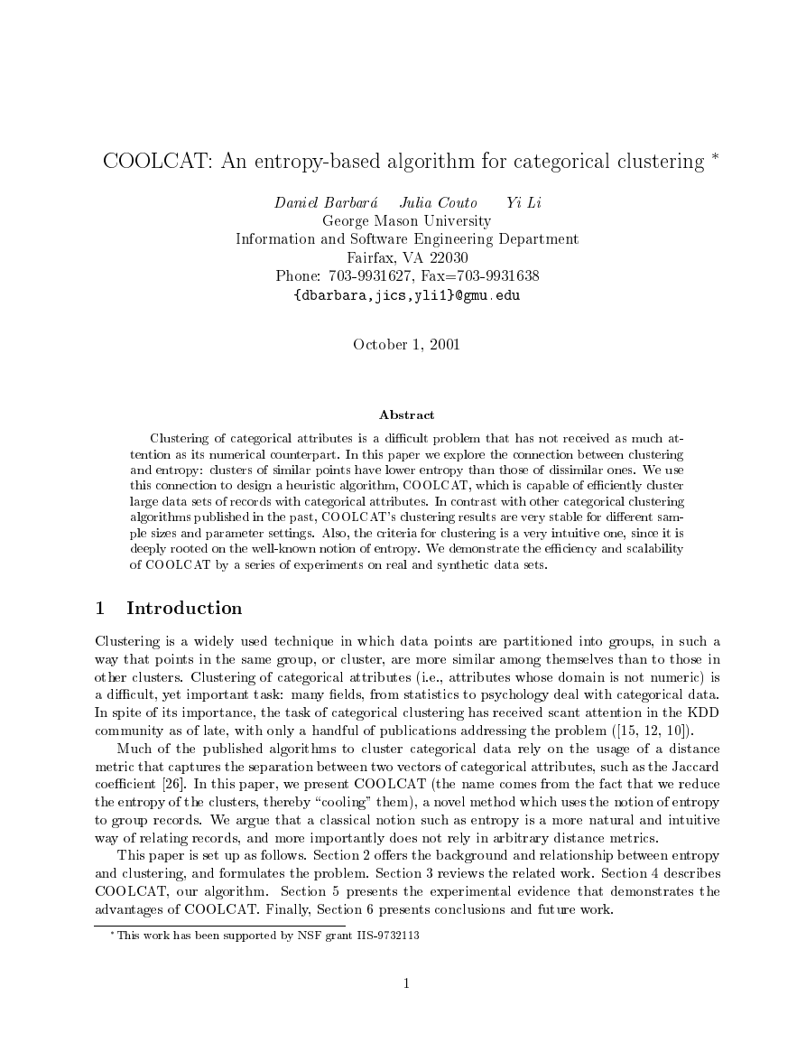
Cluster
#
Clustering �
Clustering �
Clustering �
members
Cluster� f"red"; "heavy"g
f"red"; "medium"g
E
�.�
Cluster� f"blue"; "light"g
�
members
f"red"; "heavy"g
f"blue"; "light"g
f"red"; "medium"g �
E
�:�
Members
f"red"; heavy"g
E
�
f"red"; "medium"g �:�
f"blue"; "light"g
Exp.E
�:��
�:��
�:��
Figure �: Three dierent clusterings for the set v�; v�; v�. Clustering � minimizes the expected
entropy of the two clusters.
Furthermore, we make a simplication in the computation of entropy of a set of records. We
assume independence of the attributes of the record, transforming Equation � into Equation �. In
other words, the joint probability of the combined attribute values becomes the product of the
probabilities of each attribute, and hence the entropy can be calculated as the sum of entropies of
the attributes.
E(^x) = X
X
(p(x�) p(xn))log(p(x�) p(xn))
x� � S(X�)
xn � S(Xn)
= E(X�) + E(X�) + + E(Xn)
(�)
Assume that we have a set of three records, v�; v� as before, and v� = f"red"; "medium"g,
and we want to form two clusters with them. Figure � shows all the possible arrangements, with
the entropy of each cluster, and the expected entropy in each arrangement. As we can see, the
minimum expected entropy is that of arrangement �, which obviously is the correct way of clustering
the records (using two clusters).
However, in the cases we can demonstrate that there is a correlation between two or more
attributes of the data set, we will change the data points by creating attributes that reect these
correlations and then apply Equation � to compute the join entropy. For instance, if the data set
is composed of records of attributes A; B; C; D; E; F and we know that A; B, A; C and E; F are
correlated. we will convert the data set into one having records with attributes AB; AC; D; EF
and compute the entropy assuming that these new attributes are independent. Notice that for the
grouped attributes, we are in eect computing their joint probabilities.
�.� Entropy and the similarity coecients
As we shall prove shortly, as a measure of the similarity between two vectors, the use of entropy
is equivalent to that of other widely-used similarity coecients [��]. Similarity coecients are best
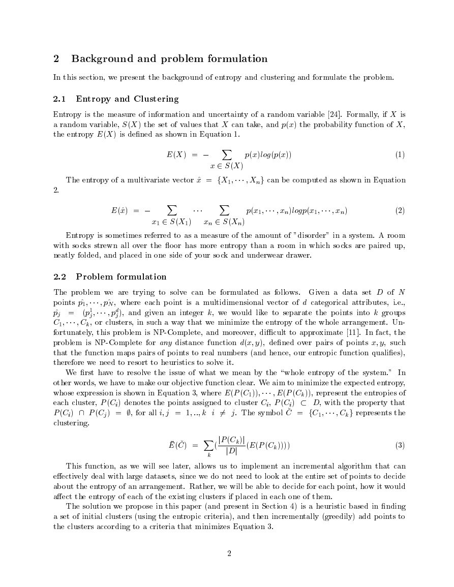
explained by the �x� association table shown in Figure �, where � refers to the presence of a variable
and � to its absence.
The simple matching coecient (SM) is dened as shown in Equation �. Notice that this coe-
cient takes into account the joint absence of a variable (as indicated by d in the table).
SM =
(a + d)
(a + b + c + d)
�
(�)
�
�
a
c
�
b
d
�
�
Figure �: Association table: � refers to the presence of a variable, and � to its absence.
The Jaccard (J) coecient is shown in Equation �. It avoids the use of joint absences of a variable
in the calculation of similarity.
Lemma � For any vectors p; q; u; v in a data set, SM (fp; qg) = SM (fu; vg) i E(fp; qg) =
J =
a
(a + b + c)
(�)
E(fu; vg).
Proof: Throughout the proof, we will use SM (fp; qg =
a� + d�
a� + b� + c� + d�
and SM (fu; vg) =
a� + d�
where a�; b�; c�; d� are the entries of the association table of p; q, and a�; b�; c�; d�
a� + b� + c� + d�
those for the association table of u; v. Notice that since the vectors are drawn from the same data
set, they all have the same number of attributes, therefore, a� + b� + c� + d� = a� + b� + c� + d�.
We shall proceed with the proof of the two implications.
Part a) If SM (fp; qg) = SM (fu; vg), then E(fp; qg) = E(fu; vg):
Since SM (fp; qg) = SM (fu; vg) = k, then a� + d� = k(a� + b� + c� + d�) and a� + d� =
k(a� + b� + c� + d�). Also, since a� + b� + c� + d� = a� + b� + c� + d�, it follows that a� + d� = a� + d�,
and b� + c� = b� + c�. Now, since for matching attributes, the entropy contribution will be �,
and for non-matching attributes, the entropy contribution will be (� �
� )), then it follows that
E(fp; qg) = (b� + c�)log( �
� ) = (b� + c�)log( �
� ) = E(fu; vg).
� log( �
Part b) If E(fp; qg) = E(fu; vg), then SM (fp; qg) = SM (fu; vg): Since for any pair of vectors,
the matching attributes will not contribute to the total entropy, while the non-matching attributes
will contribute log( �
� ) (i.e., an equal amount per attribute), then E(fp; qg) = E(fu; vg) implies that
b� + c� = b� + c�. Now, since a� + b� + c� + d� = a� + b� + c� + d�, it follows that a� + d� = a� + d�
proving the implication.
Lemma � For any vectors p; q; u; v in a data set, SM (fp; qg) > SM (fu; vg) i E(fp; qg) <
E(fu; vg).
Proof: Part a) If SM (fp; qg) > SM (fu; vg) then E(fp; qg) < E(fu; vg).
Since the rst coecient is larger than the second, it means that more attribute values agree for
the two vectors (a� + d� > a� + d�). This, obviously reduces the entropy of the pair, since agreeing
values contribute with � to the nal entropy count.
Part b) If E(fp; qg) < E(fu; vg), then SM (fp; qg) > SM (fu; vg).
Since the entropy of the rst pair is less than that of the second, it means that less attributes in
� )), i.e., b� + c� < b� + c�. Therefore,
the vectors disagree (since those contribute with the value log( �
the coecient will be larger (more values agree).
Lemma � For any vectors p; q; u; v in a data set, SM (fp; qg) < SM (fu; vg) i E(fp; qg) >
E(fu; vg).
Proof: Similar to Lemma �.
Theorem � Given two similarity matrices built over the same data set, one using SM and the
�
�
�
�
�
�
�
�
�
�
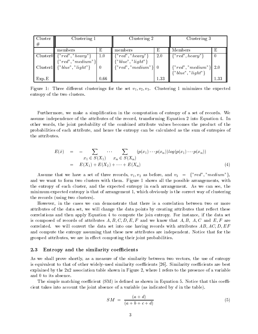
Figure �: Association table for vectors v� = �; �; � and v� = �; �; �.
other entropy, if we order the rst matrix in descending order of entries, and the second in ascending
order, the relative ordering of the pairs of points is the same in both cases.
Proof: By Lemmas �, � and �.
As a consequence of Theorem �, in any algorithm that uses the SM coecient as a similarity
measure, we could also use entropy as well, obtaining identical results. For instance, ROCK [��]
(which we shall review in Section �) uses an \extended" similarity measure in which the coecient
is computed as the number of attributes that agree divided by the total number of attribute val-
ues, calling this coecient the Jaccard coecient. (For instance, in the example shown in Section
�.�, the coecient J(fv�; v�g) = �, since no values are the same in v� = < red; heavy > and
v� = < blue; light >; but J(fv�; v�g) = �
� , since one value out of three is the same in the pair
v� = < red; heavy >, v� = f"red"; "medium"g.)
In fact, it is easy to see that if we convert
the "red", "heavy", and "medium" values into binary variables, the vectors become v� = �; �; �
and v� = �; �; �, and the association table for v�; v� is the one shown in Figure �. Then the SM
coecient can be easily computed as �
� . The Jaccard coecient in this case would also be the same,
as d = �. This fact is true for every case in which we convert the values into binary variables since
we will never have a column in which the two binary values are �. So, it is easy to see that Theorem
� will always apply when the Jaccard coecient is applied to nominal attributes by converting the
values to binary variables, since then the Jaccard coecient and the SM coecient would be equal.
Our algorithm, COOLCAT, however, uses the fact that entropy, unlike the SM or Jaccard coef-
cients, can serve as a measure of similarity among any set of vectors (not just two).
�.� Expected entropy and the Minimum Description Length principle
The Minimum Description Length principle (MDL) [��, ��] recommends choosing the model that
minimizes the number of bits needed to encode it. This principle is widely used to compare classiers
(see [��]) but it has not been used much to deal with clustering. (An idea of how to do this by encoding
the clusters centers is sketched in [��]).
An optimal encoding for a set of clusters can be realized by assigning codes to each attribute of
the data based on the probability that the attribute appears on the cluster, using a Homan code.
This encoding will have length Pi P (Ai = Vij)logP (Ai = Vij) for each cluster Ck. So, it can be
minimized by minimizing the expected value of that function. But, this is precisely the function we
have selected to minimize: the expected entropy of the clustering. So, our technique aims to nd
the clustering that follows the MDL principle. This has important implications: the fact that the
encoding of the clusters is minimal implies that we can expect very concise representations of the
clusters we have found at any given point. This in turn makes possible the incremental processing
of further data points without having to keep all the previous data points in memory, but just the
concise representation of the clusters they form.
�
�
f�; �; �g
f�; �; �g
f�; �; �g
f�; �; �g
f�; �; �g
f�; �; �g
f�; �; �g
f�; �; �g
f�; �; �g
f�; �; �g
f�; �; �g
f�; �; �g
f�; �; �g
f�; �; �g
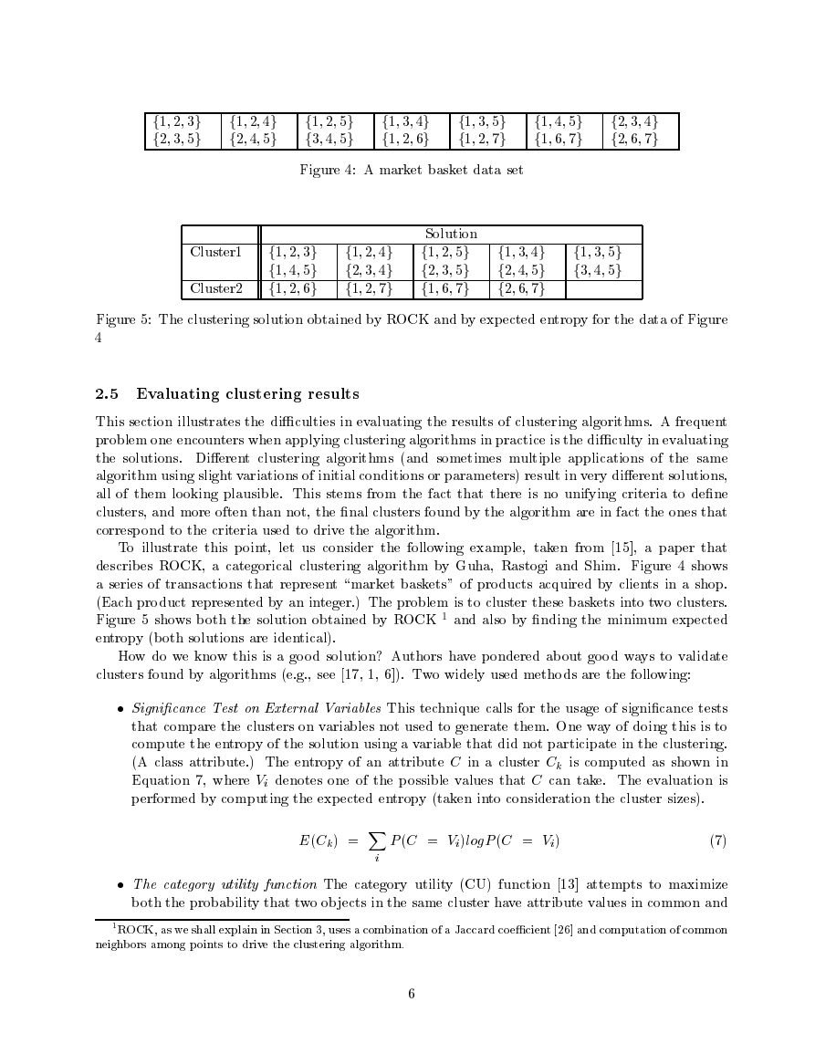
Figure �: A market basket data set
Cluster�
Cluster�
f�; �; �g
f�; �; �g
f�; �; �g
f�; �; �g
f�; �; �g
f�; �; �g
Solution
f�; �; �g
f�; �; �g
f�; �; �g
f�; �; �g
f�; �; �g
f�; �; �g
f�; �; �g
f�; �; �g
Figure �: The clustering solution obtained by ROCK and by expected entropy for the data of Figure
�
�.� Evaluating clustering results
This section illustrates the diculties in evaluating the results of clustering algorithms. A frequent
problem one encounters when applying clustering algorithms in practice is the diculty in evaluating
the solutions. Dierent clustering algorithms (and sometimes multiple applications of the same
algorithm using slight variations of initial conditions or parameters) result in very dierent solutions,
all of them looking plausible. This stems from the fact that there is no unifying criteria to dene
clusters, and more often than not, the nal clusters found by the algorithm are in fact the ones that
correspond to the criteria used to drive the algorithm.
To illustrate this point, let us consider the following example, taken from [��], a paper that
describes ROCK, a categorical clustering algorithm by Guha, Rastogi and Shim. Figure � shows
a series of transactions that represent \market baskets" of products acquired by clients in a shop.
(Each product represented by an integer.) The problem is to cluster these baskets into two clusters.
Figure � shows both the solution obtained by ROCK � and also by nding the minimum expected
entropy (both solutions are identical).
How do we know this is a good solution? Authors have pondered about good ways to validate
clusters found by algorithms (e.g., see [��, �, �]). Two widely used methods are the following:
Signicance Test on External Variables This technique calls for the usage of signicance tests
that compare the clusters on variables not used to generate them. One way of doing this is to
compute the entropy of the solution using a variable that did not participate in the clustering.
(A class attribute.) The entropy of an attribute C in a cluster Ck is computed as shown in
Equation �, where Vi denotes one of the possible values that C can take. The evaluation is
performed by computing the expected entropy (taken into consideration the cluster sizes).
E(Ck) = X
i
P (C = Vi)logP (C = Vi)
(�)
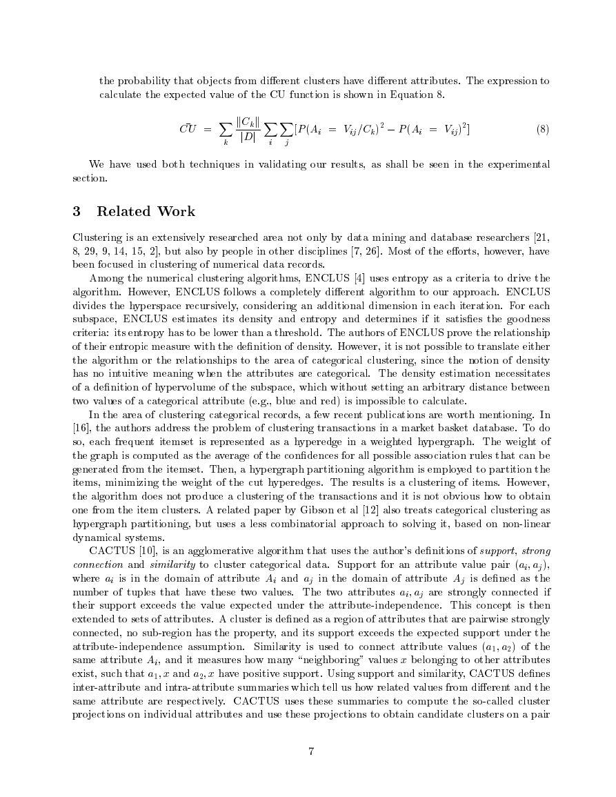
The category utility function The category utility (CU) function [��] attempts to maximize
both the probability that two objects in the same cluster have attribute values in common and
�ROCK, as we shall explain in Section �, uses a combination of a Jaccard coecient [��] and computation of common
neighbors among points to drive the clustering algorithm.
�
�
the probability that objects from dierent clusters have dierent attributes. The expression to
calculate the expected value of the CU function is shown in Equation �.
CU = X
k
kCkk
jDj
X
i
X
j
[P (Ai = Vij=Ck)� P (Ai = Vij)�]
(�)
We have used both techniques in validating our results, as shall be seen in the experimental
section.
� Related Work
Clustering is an extensively researched area not only by data mining and database researchers [��,
�, � , , ��, ��, �], but also by people in other disciplines [�, ��]. Most of the eorts, however, have
been focused in clustering of numerical data records.
Among the numerical clustering algorithms, ENCLUS [�] uses entropy as a criteria to drive the
algorithm. However, ENCLUS follows a completely dierent algorithm to our approach. ENCLUS
divides the hyperspace recursively, considering an additional dimension in each iteration. For each
subspace, ENCLUS estimates its density and entropy and determines if it satises the goodness
criteria: its entropy has to be lower than a threshold. The authors of ENCLUS prove the relationship
of their entropic measure with the denition of density. However, it is not possible to translate either
the algorithm or the relationships to the area of categorical clustering, since the notion of density
has no intuitive meaning when the attributes are categorical. The density estimation necessitates
of a denition of hypervolume of the subspace, which without setting an arbitrary distance between
two values of a categorical attribute (e.g., blue and red) is impossible to calculate.
In the area of clustering categorical records, a few recent publications are worth mentioning. In
[��], the authors address the problem of clustering transactions in a market basket database. To do
so, each frequent itemset is represented as a hyperedge in a weighted hypergraph. The weight of
the graph is computed as the average of the condences for all possible association rules that can be
generated from the itemset. Then, a hypergraph partitioning algorithm is employed to partition the
items, minimizing the weight of the cut hyperedges. The results is a clustering of items. However,
the algorithm does not produce a clustering of the transactions and it is not obvious how to obtain
one from the item clusters. A related paper by Gibson et al [��] also treats categorical clustering as
hypergraph partitioning, but uses a less combinatorial approach to solving it, based on non-linear
dynamical systems.
CACTUS [��], is an agglomerative algorithm that uses the author’s denitions of support, strong
connection and similarity to cluster categorical data. Support for an attribute value pair (ai; aj),
where ai is in the domain of attribute Ai and aj in the domain of attribute Aj is dened as the
number of tuples that have these two values. The two attributes ai; aj are strongly connected if
their support exceeds the value expected under the attribute-independence. This concept is then
extended to sets of attributes. A cluster is dened as a region of attributes that are pairwise strongly
connected, no sub-region has the property, and its support exceeds the expected support under the
attribute-independence assumption. Similarity is used to connect attribute values (a�; a�) of the
same attribute Ai, and it measures how many \neighboring" values x belonging to other attributes
exist, such that a�; x and a�; x have positive support. Using support and similarity, CACTUS denes
inter-attribute and intra-attribute summaries which tell us how related values from dierent and the
same attribute are respectively. CACTUS uses these summaries to compute the so-called cluster
projections on individual attributes and use these projections to obtain candidate clusters on a pair
�
�
Hierarchical agglomerative methods (e.g.,
of attributes, extending then to three and more attributes. CACTUS, obviously, bases its clustering
decisions on the \neighboring" concept of similarity, similar to the algorithms described in [��, ��].
[��, � , ��]), cluster points by iteratively merging
clusters (at the start every point is a cluster by itself). For instance, the single linkage method [��]
begins searching for the two most similar points in a similarity matrix and puts them in the same
cluster. Then it searches for the most similar point to those in the cluster, making this point part
of the cluster. At every step, the algorithm looks for points to join into existing clusters (or among
themselves). The problem with agglomerative methods is that they do not scale, since they require
the calculation and storage of potentially large similarity matrices. They also lack stability when the
data is re-shued in the similarity matrix.
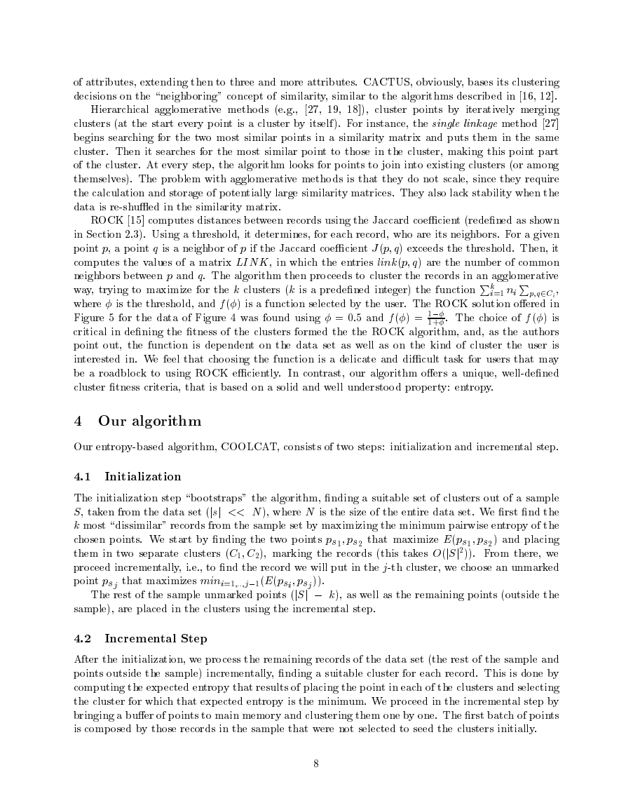
ROCK [��] computes distances between records using the Jaccard coecient (redened as shown
in Section �.�). Using a threshold, it determines, for each record, who are its neighbors. For a given
point p, a point q is a neighbor of p if the Jaccard coecient J(p; q) exceeds the threshold. Then, it
computes the values of a matrix LIN K, in which the entries link(p; q) are the number of common
neighbors between p and q. The algorithm then proceeds to cluster the records in an agglomerative
way, trying to maximize for the k clusters (k is a predened integer) the function Pk
i=� ni Pp;q�Ci,
where is the threshold, and f () is a function selected by the user. The ROCK solution oered in
Figure � for the data of Figure � was found using = �:� and f () = �
�+ . The choice of f () is
critical in dening the tness of the clusters formed the the ROCK algorithm, and, as the authors
point out, the function is dependent on the data set as well as on the kind of cluster the user is
interested in. We feel that choosing the function is a delicate and dicult task for users that may
be a roadblock to using ROCK eciently. In contrast, our algorithm oers a unique, well-dened
cluster tness criteria, that is based on a solid and well understood property: entropy.
� Our algorithm
Our entropy-based algorithm, COOLCAT, consists of two steps: initialization and incremental step.
�.�
Initialization
The initialization step \bootstraps" the algorithm, nding a suitable set of clusters out of a sample
S, taken from the data set (jsj << N ), where N is the size of the entire data set. We rst nd the
k most \dissimilar" records from the sample set by maximizing the minimum pairwise entropy of the
chosen points. We start by nding the two points ps�; ps� that maximize E(ps�; ps�) and placing
them in two separate clusters (C�; C�), marking the records (this takes O(jSj�)). From there, we
proceed incrementally, i.e., to nd the record we will put in the j-th cluster, we choose an unmarked
point psj that maximizes mini=�;::;j�(E(psi; psj )).
The rest of the sample unmarked points (jSj k), as well as the remaining points (outside the
sample), are placed in the clusters using the incremental step.
�.�
Incremental Step
After the initialization, we process the remaining records of the data set (the rest of the sample and
points outside the sample) incrementally, nding a suitable cluster for each record. This is done by
computing the expected entropy that results of placing the point in each of the clusters and selecting
the cluster for which that expected entropy is the minimum. We proceed in the incremental step by
bringing a buer of points to main memory and clustering them one by one. The rst batch of points
is composed by those records in the sample that were not selected to seed the clusters initially.
�
�



 2023年江西萍乡中考道德与法治真题及答案.doc
 2012年重庆南川中考生物真题及答案.doc
 2013年江西师范大学地理学综合及文艺理论基础考研真题.doc
 2020年四川甘孜小升初语文真题及答案I卷.doc
 2020年注册岩土工程师专业基础考试真题及答案.doc
 2023-2024学年福建省厦门市九年级上学期数学月考试题及答案.doc
 2021-2022学年辽宁省沈阳市大东区九年级上学期语文期末试题及答案.doc
 2022-2023学年北京东城区初三第一学期物理期末试卷及答案.doc
 2018上半年江西教师资格初中地理学科知识与教学能力真题及答案.doc
 2012年河北国家公务员申论考试真题及答案-省级.doc
 2020-2021学年江苏省扬州市江都区邵樊片九年级上学期数学第一次质量检测试题及答案.doc
 2022下半年黑龙江教师资格证中学综合素质真题及答案.doc