8
0
0
2
l
u
J
1
]
G
L
.
s
c
[
1
v
3
9
0
0
.
7
0
8
0
:
v
i
X
r
a
Journal of Machine Learning Research 9 (2008) 1–41
Submitted 05/08; Published xx/08
Graph Kernels
SVN.Vishwanathan@nicta.com.au
kmb51@cam.ac.uk
risi@gatsby.ucl.ac.uk
jmlr@schraudolph.org
S.V. N. Vishwanathan
College of Engineering and Computer Science
Australian National University and NICTA
Locked Bag 8001, Canberra ACT 2601, Australia
Karsten M. Borgwardt
Machine Learning Group, Department of Engineering
University of Cambridge
Trumpington Street, CB2 1PZ Cambridge, United Kingdom
Imre Risi Kondor
Gatsby Computational Neuroscience Unit
University College London
17 Queen Square, WC1N 3AR London, United Kingdom
Nicol N. Schraudolph
College of Engineering and Computer Science
Australian National University and NICTA
Locked Bag 8001, Canberra ACT 2601, Australia
Editor: U. N. Known
Abstract
We present a unified framework to study graph kernels, special cases of which include
the random walk graph kernel (G¨artner et al., 2003; Borgwardt et al., 2005), marginal-
ized graph kernel (Kashima et al., 2003, 2004; Mah´e et al., 2004), and geometric kernel
on graphs (G¨artner, 2002). Through extensions of linear algebra to Reproducing Kernel
Hilbert Spaces (RKHS) and reduction to a Sylvester equation, we construct an algorithm
that improves the time complexity of kernel computation from O(n6) to O(n3). When
the graphs are sparse, conjugate gradient solvers or fixed-point iterations bring our algo-
rithm into the sub-cubic domain. Experiments on graphs from bioinformatics and other
application domains show that it is often more than a thousand times faster than previous
approaches. We then explore connections between diffusion kernels (Kondor and Lafferty,
2002), regularization on graphs (Smola and Kondor, 2003), and graph kernels, and use
these connections to propose new graph kernels. Finally, we show that rational kernels
(Cortes et al., 2002, 2003, 2004) when specialized to graphs reduce to the random walk
graph kernel.
Keywords: Graph kernels, Linear Algebra in RKHS, Sylvester Equations, Bioinformatics,
Rational Kernels, Transducers, Semirings, Diffusion, Random Walks, Regularization on
Graphs.
c2008 S.V. N. Vishwanathan, Karsten M. Borgwardt, Imre Risi Kondor, and Nicol N. Schraudolph.
�
Vishwanathan, Borgwardt, Kondor, and Schraudolph
1. Introduction
We begin by providing some background, establishing some basic notation, and giving an
outline of the paper.
1.1 Background
Machine learning in domains such as bioinformatics (Sharan and Ideker, 2006), chemoin-
formatics (Bonchev and Rouvray, 1991), drug discovery (Kubinyi, 2003), web data mining
(Washio and Motoda, 2003), and social networks (Kumar et al., 2006) involves the study
of relationships between structured objects. Graphs are natural data structures to model
such structures, with nodes representing objects and edges the relations between them. In
this context, one often encounters two questions: “How similar are two nodes in a given
graph?” and “How similar are two graphs to each other?”
Kernel methods (Sch¨olkopf and Smola, 2002) offer a natural framework to study these
questions. Roughly speaking, a kernel k(x, x) is a measure of similarity between objects
x and x. It must satisfy two mathematical requirements: it must be symmetric, that is,
k(x, x) = k(x, x), and positive semi-definite (p.s.d.). Comparing nodes in a graph involves
constructing a kernel between nodes, while comparing graphs involves constructing a kernel
between graphs. In both cases, the challenge is to define a kernel that captures the semantics
inherent in the graph structure but at the same time is reasonably efficient to evaluate.
Until now, the above two types of kernels have largely been studied separately. The
idea of constructing kernels on graphs (i.e., between the nodes of a single graph) was
first proposed by Kondor and Lafferty (2002), and extended by Smola and Kondor (2003).
Kernels between graphs were proposed by G¨artner (2002) (geometric kernels on graphs)
and G¨artner et al. (2003) (random walk graph kernels), and later extended by Borgwardt
et al. (2005). Much at the same time, the idea of marginalized kernels (Tsuda et al., 2002)
was extended to graphs by Kashima et al. (2003, 2004), and further refined by Mah´e et al.
(2004). A seemingly independent line of research investigates the so-called rational kernels,
which are kernels between finite state automata based on the algebra of abstract semirings
(Cortes et al., 2004, 2003, 2002).
The aim of this paper is twofold: on one hand we present theoretical results showing
that these four strands of research are in fact closely related, on the other we present
new algorithms for efficiently computing kernels between graphs. Towards this end we first
establish some notation and review pertinent concepts from linear algebra and graph theory.
1.2 Linear Algebra Concepts
We use ei to denote the ith standard basis vector (that is, a vector of all zeros with the ith
entry set to one), e to denote a vector with all entries set to one, 0 to denote the vector
of all zeros, and I to denote the identity matrix. When it is clear from context we will not
mention the dimensions of these vectors and matrices.
2
�
Graph Kernels
Definition 1 Given real matrices A ∈ Rn×m and B ∈ Rp×q, the Kronecker product A⊗B ∈
Rnp×mq and column-stacking operator vec(A) ∈ Rnm are defined as
A11B A12B . . . A1mB
...
...
...
...
A ⊗ B :=
, vec(A) :=
A∗1
...
A∗m
,
An1B An2B . . . AnmB
where A∗j denotes the jth column of A.
Kronecker product and vec operator are linked by the well-known property (e.g., Bernstein,
2005, proposition 7.1.9):
vec(ABC) = (C⊗ A) vec(B).
(1)
Another well-known property of the Kronecker product, which we use in Section 5, is
(Bernstein, 2005, proposition 7.1.6):
(A ⊗ B)(C ⊗ D) = AC ⊗ BD.
(2)
A closely related concept is that of the Kronecker sum which is defined for real matrices
A ∈ Rn×m and B ∈ Rp×q as
A ⊕ B := A ⊗ Ipq + Inm ⊗ B,
(3)
with Inm (resp. Ipq) denoting the n× m (resp. p× q) identity matrix. Many of its properties
can be derived from those of the Kronecker product.
Finally, the Hadamard product of two real matrices A, B ∈ Rn×m, denoted by A B ∈
Rn×m, is obtained by element-wise multiplication. It interacts with the Kronecker product
via
(A ⊗ B) (C ⊗ D) = (A C) ⊗ (B D).
(4)
All the above concepts can be extended to a Reproducing Kernel Hilbert Space (RKHS)
(See Appendix A for details).
1.3 Graph Concepts
A graph G consists of an ordered set of n vertices V = {v1, v2, . . . , vn}, and a set of edges
E ⊂ V × V . A vertex vi is said to be a neighbor of another vertex vj if they are connected
by an edge, i.e., if (vi, vj) ∈ E; this is also denoted vi ∼ vj. A walk of length t on G
is a sequence of indices i1, i2, . . . it+1 such that vik ∼ vik+1 for all 1 ≤ k ≤ t. A graph
is said to be connected if any two pairs of vertices can be connected by a walk. In this
paper we will always work with connected graphs. A graph is said to be undirected if
(vi, vj) ∈ E ⇐⇒ (vj, vi) ∈ E.
In much of the following we will be dealing with weighted graphs, which are a slight
In a weighted graph, each edge (vi, vj) has an associated
generalization of the above.
weight wij > 0 signifying its “strength”. If vi and vj are not neighbors, then wij = 0. In
an undirected weighted graph wij = wji.
3
�
Vishwanathan, Borgwardt, Kondor, and Schraudolph
vi ∼ vj, and 0 otherwise. The adjacency matrix of a weighted graph is just the matrix
In both cases, if G is undirected, then the adjacency matrix is
The adjacency matrix of an unweighted graph is an n × n matrix A with Aij = 1 if
of weights, Aij = wij.
symmetric. The diagonal entries of A are always zero.
The adjacency matrix has a normalized cousin, defined A := D−1A, which has the
Dii = di =
property that each of its rows sums to one, therefore it can serve as the transition matrix
jAij. A random walk on G is a process generating sequences of vertices
for a stochastic process. Here, D is a diagonal matrix of node degrees, di, such that
vi1, vi2, vi3, . . . according to P(ik+1|i1, . . . ik) = Aik,ik+1, that is, the probability at vik of
picking vik+1 next is proportional to the weight of the edge (vik , vik+1). The tth power of
A thus describes t-length walks, i.e., [At]ij is the probability of a transition from vertex vi
to vertex vj via a walk of length t. If p0 is an initial probability distribution over vertices,
the probability distribution pt describing the location of our random walker at time t is
pt = Atp0. The jth component of pt denotes the probability of finishing a t-length walk at
vertex vj. We will use this intuition to define generalized random walk graph kernels.
Let X be a set of labels which includes the special label ζ. Every edge-labeled graph G
is associated with a label matrix X ∈ X n×n such that Xij = ζ iff (vi, vj) /∈ E, in other words
only those edges which are present in the graph get a non-ζ label. Let H be the RKHS
endowed with the kernel κ : X ×X → R, and let φ : X → H denote the corresponding
feature map which maps ζ to the zero element of H. We use Φ(X) to denote the feature
matrix of G (see Appendix A for details). For ease of exposition we do not consider labels
on vertices here, though our results hold for that case as well. Henceforth we use the term
labeled graph to denote an edge-labeled graph.
1.4 Paper Outline
In the first part of this paper (Sections 2–4) we present a unifying framework for graph
kernels, encompassing many known kernels as special cases, and connecting to others. We
describe our framework in Section 2, prove that it leads to p.s.d. kernels, and discuss
random walk graph kernels, geometric kernels on graphs, and marginalized graph kernels
as special cases. For ease of exposition we will work with real matrices in the main body
of the paper and relegate the RKHS extensions to Appendix A. In Section 3 we present
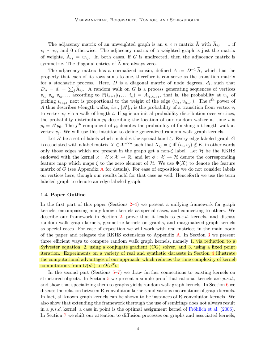
three efficient ways to compute random walk graph kernels, namely 1. via reduction to a
Sylvester equation, 2. using a conjugate gradient (CG) solver, and 3. using a fixed point
iteration. Experiments on a variety of real and synthetic datasets in Section 4 illustrate
the computational advantages of our approach, which reduces the time complexity of kernel
computations from O(n6) to O(n3).
In the second part (Sections 5–7) we draw further connections to existing kernels on
structured objects. In Section 5 we present a simple proof that rational kernels are p.s.d.,
and show that specializing them to graphs yields random walk graph kernels. In Section 6 we
discuss the relation between R-convolution kernels and various incarnations of graph kernels.
In fact, all known graph kernels can be shown to be instances of R-convolution kernels. We
also show that extending the framework therough the use of semirings does not always result
in a p.s.d. kernel; a case in point is the optimal assignment kernel of Fr¨ohlich et al. (2006).
In Section 7 we shift our attention to diffusion processes on graphs and associated kernels;
4
�
Graph Kernels
this leads us to propose new kernels on graphs, based on the Cartesian graph product. We
show that the efficient computation techniques we introduced in Section 3 are also applicable
here, but are ultimately forced to conclude that diffusion-based graph kernels are not useful
in a general context. We conclude in Section 8 with an outlook and discussion.
2. Random Walk Graph Kernels
Our generalized random walk graph kernels are based on a simple idea: given a pair of
graphs, perform random walks on both, and count the number of matching walks. We show
that this simple concept underlies random walk graph kernels, marginalized graph kernels,
and geometric kernels on graphs.
In order to do this, we first need to introduce direct
product graphs.
2.1 Direct Product Graphs
Given two graphs G(V, E) and G(V , E)(with |V | = n and |V | = n), their direct product
G× is a graph with vertex set
V× = {(vi, v
i) : vi ∈ V, v
i ∈ V },
(5)
and edge set
E× = {((vi,v
j)) : (vi, vj)∈ E ∧ (v
(6)
In other words, G× is a graph over pairs of vertices from G and G, and two vertices in G×
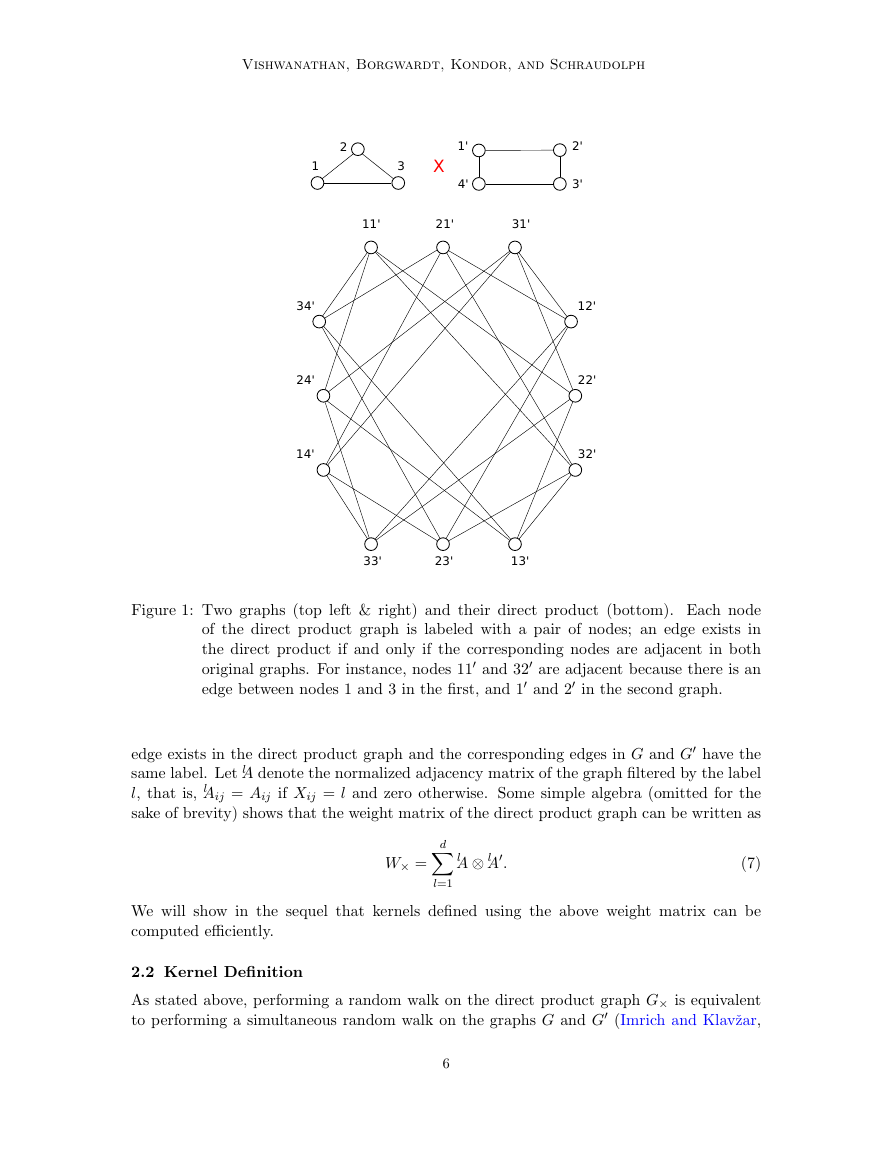
are neighbors if and only if the corresponding vertices in G and G are both neighbors (see
are the respective adjacency matrices of G and
i), (vj,v
Figure 1 for an illustration). If A and A
G, then the adjacency matrix of G× is A× = A⊗A
. Similarly, A× = A ⊗ A.
i, v
j)∈ E}.
If G and G are edge-labeled, we can associate a weight matrix W× ∈ Rnn×nn
Performing a random walk on the direct product graph is equivalent to performing a
simultaneous random walk on G and G (Imrich and Klavˇzar, 2000). If p and p denote
initial probability distributions over the vertices of G and G, then the corresponding initial
probability distribution on the direct product graph is p× := p⊗ p. Likewise, if q and q are
stopping probabilities (that is, the probability that a random walk ends at a given vertex),
then the stopping probability on the direct product graph is q× := q ⊗ q.
with
G× using our Kronecker product in RKHS (Definition 12): W× = Φ(X) ⊗ Φ(X). As a
consequence of the definition of Φ(X) and Φ(X), the entries of W× are non-zero only if
the corresponding edge exists in the direct product graph. The weight matrix is closely
related to the normalized adjacency matrix: assume that H = R endowed with the usual
inner product, and φ(Xij) = 1/di if (vi, vj) ∈ E or zero otherwise. Then Φ(X) = A and
Φ(X) = A, and consequently W× = A×, that is, the weight matrix is identical to the
normalized adjacency matrix of the direct product graph.
To extend the above discussion, assume that H = Rd endowed with the usual inner
product, and that there are d distinct edge labels {1, 2, . . . , d}. For each edge (vi, vj) ∈ E
we have φ(Xij) = el /di if the edge (vi, vj) is labeled l. All other entries of Φ(X) are set to
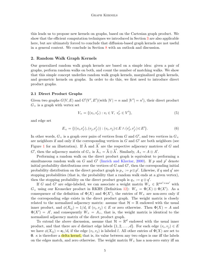
0. κ is therefore a delta kernel, that is, its value between any two edges is one iff the labels
on the edges match, and zero otherwise. The weight matrix W× has a non-zero entry iff an
5
�
Vishwanathan, Borgwardt, Kondor, and Schraudolph
Figure 1: Two graphs (top left & right) and their direct product (bottom). Each node
of the direct product graph is labeled with a pair of nodes; an edge exists in
the direct product if and only if the corresponding nodes are adjacent in both
original graphs. For instance, nodes 11 and 32 are adjacent because there is an
edge between nodes 1 and 3 in the first, and 1 and 2 in the second graph.
edge exists in the direct product graph and the corresponding edges in G and G have the
same label. Let lA denote the normalized adjacency matrix of the graph filtered by the label
l, that is, lAij = Aij if Xij = l and zero otherwise. Some simple algebra (omitted for the
sake of brevity) shows that the weight matrix of the direct product graph can be written as
d
W× =
lA ⊗ lA.
(7)
We will show in the sequel that kernels defined using the above weight matrix can be
computed efficiently.
l=1
2.2 Kernel Definition
As stated above, performing a random walk on the direct product graph G× is equivalent
to performing a simultaneous random walk on the graphs G and G (Imrich and Klavˇzar,
6
11'21'31'34'24'14'12'22'32'13'23'33'1231'2'3'4'X�
Graph Kernels
2000). Therefore, the ((i − 1)n + j, (i − 1)n + j)th entry of Ak× represents the probability
of simultaneous k length random walks on G (starting from vertex vi and ending in vertex
vj) and G (starting from vertex v
j). The entries of W× represent
similarity between edges. The ((i − 1)n + j, (i − 1)n + j)th entry of W k× represents the
similarity between simultaneous k length random walks on G and G measured via the
kernel function κ.
and an appropriately chosen discrete measure µ, we can define a kernel on G and G as
Given the weight matrix W×, initial and stopping probability distributions p× and q×,
i and ending in vertex v
k(G, G) :=
µ(k) q
×W k×p×.
(8)
∞
k=1
In order to show that (8) is a valid p.s.d. kernel we need the following technical lemma:
∀ k ∈ N : W k×p× = vec[Φ(X)kp (Φ(X)kp)].
Lemma 2
Proof By induction over k. Base case: k = 1. Observe that
p× = (p ⊗ p) vec(1) = vec(pp).
(9)
By using Lemma 13, W×p× can be written as
[Φ(X) ⊗ Φ(X)] vec(pp) = vec[Φ(X)ppΦ(X)]
= vec[Φ(X)p(Φ(X)p)].
(10)
Induction from k to k+1: Using the induction assumption W k×p× = vec[Φ(X)kp (Φ(X)kp)]
and Lemma 13 we obtain
W k+1× p× = W×W k×p× = (Φ(X) ⊗ Φ(X)) vec[Φ(X)kp (Φ(X)kp)]
= vec[Φ(X)Φ(X)kp (Φ(X)kp)Φ(X)]
= vec[Φ(X)k+1p (Φ(X)k+1p)].
(11)
Lemma 3 If the measure µ(k) is such that (8) converges, then it defines a valid p.s.d.
kernel.
Proof Using Lemmas 13 and 2 we can write
×W k×p× = (q ⊗ q) vec[Φ(X)kp (Φ(X)kp)]
q
= vec[qΦ(X)kp (Φ(X)kp)q]
= (qΦ(X)kp)
(qΦ(X)kp)
.
ρ(G)
ρ(G)
(12)
Each individual term of (8) equals ρ(G)ρ(G) for some function ρ, and is therefore a valid
p.s.d. kernel. The lemma follows because the class of p.s.d. kernels is closed under convex
combinations (Berg et al., 1984).
7
�
Vishwanathan, Borgwardt, Kondor, and Schraudolph
2.3 Special Cases
A popular choice to ensure convergence of (8) is to assume µ(k) = λk for some λ > 0. If λ
is sufficiently small1 then (8) is well-defined, and we can write
λkq
×W k×p× = q
×(I−λW×)−1p×.
(13)
k(G, G) =
k
Kashima et al. (2004) use marginalization and probabilities of random walks to define
kernels on graphs. Given transition probability matrices P and P associated with graphs
G and G respectively, their kernel can be written as (Kashima et al., 2004, Eq. 1.19)
k(G, G) = q
×(I−T×)−1p×,
where T× := [vec(P ) vec(P )] [Φ(X) ⊗ Φ(X)]. The edge kernel ˆκ(Xij, X
PijP
ijκ(Xij, X
G¨artner et al. (2003), on the other hand, use the adjacency matrix of the direct product
i,j) with λ=1 recovers (13).
graph to define the so-called random walk graph kernel
(14)
ij) :=
k(G, G) =
n
n
∞
i=1
j=1
k=1
λk[Ak×]ij.
(15)
n
n
To recover their kernel in our framework, assume an uniform distribution over the vertices of
G and G, that is, set p = q = 1/n and p = q = 1/n. The initial as well as final probability
distribution over vertices of G× is given by p× = q× = e /(nn). Setting Φ(X) := A,
Φ(X) = A, and W× = A×, we can rewrite (8) to obtain
∞
k=1
k(G, G) =
λkq
×Ak×p× =
1
n2n2
n
n
∞
i=1
j=1
k=1
λk[Ak×]ij,
which recovers (15) to within a constant factor.
Finally, the so-called geometric kernel is defined as (G¨artner, 2002)
k(G, G) =
[eλA×]ij = eeλA×e,
(16)
which can be recovered in our setting by setting p = q = 1/n, p = q = 1/n, Φ(L) := A,
Φ(L) = A, and µ(k) = λk/k!.
i=1
j=1
3. Efficient Computation
Computing the kernels of G¨artner et al. (2003) and Kashima et al. (2004) essentially boil
down to inverting the matrix (I−λW×). If both G and G have n vertices, then (I−λW×)
is an n2 × n2 matrix. Given that the complexity of inverting a matrix is cubic in its
dimensions, a direct computation of (13) would require O(n6) time. In the first part of
this section we show that iterative methods, including those based on Sylvester equations,
conjugate gradients, and fixed-point iterations, can be used to speed up this computation.
Later, in Section 3.4, we show that the geometric kernel can be computed in O(n3) time.
1. The values of λ which ensure convergence depend on the spectrum of W×. See Chapter 6 of Vishwanathan
(2002) for a discussion of this issue.
8
�




 2023年江西萍乡中考道德与法治真题及答案.doc
 2012年重庆南川中考生物真题及答案.doc
 2013年江西师范大学地理学综合及文艺理论基础考研真题.doc
 2020年四川甘孜小升初语文真题及答案I卷.doc
 2020年注册岩土工程师专业基础考试真题及答案.doc
 2023-2024学年福建省厦门市九年级上学期数学月考试题及答案.doc
 2021-2022学年辽宁省沈阳市大东区九年级上学期语文期末试题及答案.doc
 2022-2023学年北京东城区初三第一学期物理期末试卷及答案.doc
 2018上半年江西教师资格初中地理学科知识与教学能力真题及答案.doc
 2012年河北国家公务员申论考试真题及答案-省级.doc
 2020-2021学年江苏省扬州市江都区邵樊片九年级上学期数学第一次质量检测试题及答案.doc
 2022下半年黑龙江教师资格证中学综合素质真题及答案.doc