贝叶斯压缩感知算法.pdf

发布时间：2022-06-08 发布人：admin 分类：说明书资料大小：0.58M 资料格式：pdf 举报版权申诉

wang514558620-6227671-4744300845407488920.pdf-第1页.png

第1页 / 共11页

wang514558620-6227671-4744300845407488920.pdf-第2页.png

第2页 / 共11页

wang514558620-6227671-4744300845407488920.pdf-第3页.png

第3页 / 共11页

wang514558620-6227671-4744300845407488920.pdf-第4页.png

第4页 / 共11页

wang514558620-6227671-4744300845407488920.pdf-第5页.png

第5页 / 共11页

wang514558620-6227671-4744300845407488920.pdf-第6页.png

第6页 / 共11页

wang514558620-6227671-4744300845407488920.pdf-第7页.png

第7页 / 共11页

wang514558620-6227671-4744300845407488920.pdf-第8页.png

第8页 / 共11页

文本预览

This full text paper was peer reviewed at the direction of IEEE Communications Society subject matter experts for publication in the IEEE DySPAN 2010 proceedings Space-time Bayesian Compressed Spectrum Sensing for Wideband Cognitive Radio Networks Zhenghao Zhang ∗ ∗+, Husheng Li+, Depeng Yang+ and Changxing Pei ∗ ISN Laboratory of Xidian University, Shaanxi, China + Department of EECS University of Tennessee, Knoxville Abstract— Wideband spectrum sensing in cognitive radio net- works remains an open challenge due to wideband spectrum acquisition implementation. Compressed spectrum sensing pro- vides a powerful approach to acquire wideband signals. We pur- pose a probabilistic Space-time Bayesian Compressed Spectrum Sensing (ST-BCSS) to combat the noise in wideband compressed spectrum sensing. We present an informative hierarchical prior probabilistic model to recover the compressed spectrum by exploiting the temporal and spatial prior information. These priori information endows the robustness of spectrum sensing subject to noise and low sampling rate. We present a probabilistic framework to address how to represent, convey and fuse multi- prior information to improve the local compressed spectrum reconstruction. Numerical simulation results demonstrate that the ST-BCSS algorithm improves the performance of compressed spectrum sensing under low sampling rate and low Signal Noise Ratio (SNR), compared with the traditional Basis Pursuit and Orthogonal Matching Pursuit algorithms. A correlation based algorithm for the detection of reconstruction failure due to non-sparse spectrum is also proposed and demonstrated using numerical simulations. I. INTRODUCTION [24] Wideband cognitive radio (CR) [1] [12] [16] has received signiﬁcant attention recently. As one of the most important tasks, wideband spectrum sensing [7] requires secondary users to capture the change of spectrum with a limited number of measurements in a wide spectrum range, subject to the contamination of noise. However, due to hardware limitation, especially constrained by the performance of front-end analog-to-digital converters (ADC), spectrum sensing in the wideband scenario still remains an open challenge [23]. [34] In recent years, Compressed Sensing (CS) [6] [8] turns out to be an effective method to address the wideband spectrum sensing [28] [29]. Typically, not all subchannels are occupied by primary users simultaneously. Therefore, with large probability, the spectrum is sparse in a single spectrum sensing period. Provided that the spectrum is sparse, CS offers a method to acquire the spectrum information by using a sub-Nyquist sampling rate . A pioneering work was done in [28] [29], where CS is exploited for wideband spectrum sensing. Each secondary user carries out a wideband spectrum compressed sampling and makes a local decision according to a certain decision rule. These local detection results are then exchanged and the local ﬁnal decision will be updated. Different types of implementation structures for compressed spectrum sensing have been proposed in [17] [19] [30] [31]. 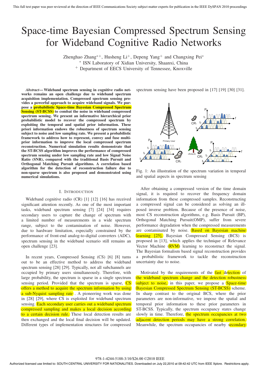P t1 t2 CR1 t3 P t1 t2 t3 Primary User P t1 f CR3 obstacle t2 CR2 t3 f f Fig. 1: An illustration of the spectrum variation in temporal and spatial aspects in spectrum sensing it is required to recover After obtaining a compressed version of the time domain signal, the frequency domain information from these compressed samples. Reconstructing a compressed signal can be considered as solving an ill- posed inverse problem. Because of the presence of noise, most CS reconstruction algorithms, e.g. Basis Pursuit (BP), Orthogonal Matching Pursuit(OMP), from severe performance degradation when the compressed measurements are contaminated by noise. Based on Bayesian machine learning [25], Bayesian Compressed Sensing (BCS) is proposed in [13], which applies the technique of Relevance Vector Machine (RVM) learning to reconstruct the signal. The Bayesian formalism based signal reconstruction provides a probabilistic framework to tackle the reconstruction uncertainty due to noise. suffer to noise, Motivated by the requirements of the fast detection of the wideband spectrum change and the detection robustness subject in this paper, we propose a Space-time Bayesian Compressed Spectrum Sensing (ST-BCSS) scheme. In sharp contrast to the original BCS, where the prior parameters are non-informative, we impose the spatial and temporal prior information to these prior parameters in ST-BCSS. Typically, the spectrum occupancy states change slowly in time. Therefore, the spectrum occupancies at two adjacent detection periods may have a strong correlation. Meanwhile, the spectrum occupancies of nearby secondary Authorized licensed use limited to: SOUTH CENTRAL UNIVERSITY FOR NATIONALITIES. Downloaded on July 22,2010 at 09:42:42 UTC from IEEE Xplore. Restrictions apply. 978-1-4244-5188-3/10/$26.00 ©2010 IEEE

This full text paper was peer reviewed at the direction of IEEE Communications Society subject matter experts for publication in the IEEE DySPAN 2010 proceedings secondary user can fuse these prior users are also highly correlated, which provides substantial spatial redundancy. Note that cooperative spectrum sensing [10] [11] [18] [33] [20] has been widely studied. However, our proposed scheme is signiﬁcantly different from existing approaches. The collaboration in our proposed algorithm is based on the technique of compressed sensing and the exchange of Bayesian priors. To efﬁciently utilize the spatial correlation, the prior information can be conveyed iteratively between two cooperative secondary users, similarly to Turbo decoding. Meanwhile, when multiple priors are provided, local information to achieve performance gain. Moreover, the information forwarding across consecutive spectrum sensing periods is also incorporated, which adds a new dimension to the redundancies. Thereby, the spatial and temporal redundancies can be jointly exploited to improve the performance of spectrum sensing. Figure 1 illustrates a wideband cooperative spectrum sensing scenario. The tower stands for a primary user. There are three secondary users carrying out cooperative spectrum sensing. And we plot a temporal-spatial spectrum graph, where the blank trapezoids represent subchannels not occupied by primary users and the solid trapezoids mean busy subchannels. From the temporal aspect, many subchannels remain the same occupancy states between two adjacent sensing periods. From the spatial aspect, CR2 is experiencing a deep shadow fading due to an obstacle between CR2 and the primary user. Therefore, the received power level at CR2 is low, compared with other secondary users. Both the temporal and spatial redundancies grant us a prior correlation information. Therefore, we can convey the spectrum detection information from the previous detection period to the current one. On the other hand, from a spatial diversity aspect, multi-agent cooperative detection [11] [18] also provides us spatial redundancy to improve the detection reliability. Similarly to Turbo Coding [2], when CR2 has only one cooperator, i.e. a nearest neighbor, the prior information can be exchanged between two cooperative secondary users. After a few iterations, it will converge to a better detection performance. The challenge of ST-BCSS is how to represent, convey information. We will and fuse the multi-agent a priori propose a mathematically elegant framework to address the challenge based on the hyperparameters of the a priori distribution of the spectrum occupancy. Moreover, a complex- valued transformation matrix is required in the spectrum reconstruction procedure since the signal in frequency domain is complex-valued. However, the existing BCS algorithms, e.g. the Fast Relevance Vector Machine (FRVM) learning algorithm [26], tackle only real-valued transformation matrices. No existing work has addressed the complex-valued case for BCS, to the authors’ best knowledge. In this paper, we extend the BCS framework into the complex-valued scenario. Moreover, we also address the problem of possibly non-sparse spectrum. When the spectrum is actually not the reconstructed spectrum may be unreliable. We sparse, exploit the spatial correction to detect the reconstruction failure to enhance the robustness of the spectrum sensing. Note that it information exchange is also considered for is signiﬁcantly compressed sensing in [3]. However, different from the ST-BCSS algorithm proposed in this paper. First, [3] applies the framework of Belief Propagation while ST-BCSS passes information via hyperparameters in the framework of Bayesian statistics. Second, in [3], the information is exchanged among different elements of the unknown vector in a way similar to the decoding of low density parity check (LDPC) codes; the information is exchanged among different secondary users and different spectrum sensing periods. Third, [3] tackles the signal reconstruction of a single user at a single snapshot while ST-BCSS deals with the collaborative spectrum sensing in multiple spectrum sensing periods. in contrast, In summary, this paper proposes a probabilistic ST-BCSS framework to combat the noise in wideband spectrum sensing. Meanwhile, it provides a novel and mathematically elegant mechanism to fuse spatial and temporal redundant informa- tion based on hyperparameter estimation and exchange. The traditional real-valued BCS is also extended to the complex ﬁeld, which is key for wideband spectrum reconstruction. The remainder of the paper is organized as follows. The wideband cognitive radio model is described in Section II. Compressed spectrum sensing and Bayesian learning are brieﬂy introduced in Section III. We present the ST-BCSS algorithm in Section IV and demonstrate the performance using numerical simula- tions in Section V. Conclusions are provided in Section VI. II. WIDEBAND COGNITIVE RADIO MODEL Suppose that there exist primary and secondary users within a wide frequency range. The entire frequency band is segmented into M non-overlapping narrowband subchan- nels. Each subchannel is labeled by its central frequency {fm} (m = 1, 2, ..., M). We assume the locations of these subchannels are preset and known. However, their power spectral density levels are varying due to the subchannel’s occupancy states of the primary users in different spectrum sensing periods. In this region, the CR network is composed of K secondary users. For simplicity, we assume that all secondary users’ spectrum sensing periods are perfectly syn- chronized, i.e. all the secondary users carry out the spectrum sensing at the same time. Thus, the k−th secondary user (k = 1, 2, ..., K) implements the binary hypotheses testing on the m-th (m = 1, 2, ...M) subchannel at sensing period t by choosing between the hypothesis H m 0,t, which means that the m-th subchannel is available, and hypothesis H m 1,t, which means that the m-th subchannel is occupied by primary users. For k-th secondary user, we deﬁne an M × 1 decision vector, m}, m = 1, 2, ..., M, to represent the denoted by Dk = {dk m-th subchannel’s usage status, which is given by dk m = 0, 1, if the m-th subchannel is occupied if the m-th subchannel is idle (1) Authorized licensed use limited to: SOUTH CENTRAL UNIVERSITY FOR NATIONALITIES. Downloaded on July 22,2010 at 09:42:42 UTC from IEEE Xplore. Restrictions apply.

This full text paper was peer reviewed at the direction of IEEE Communications Society subject matter experts for publication in the IEEE DySPAN 2010 proceedings The received signal of k-th secondary user is represented by yk(t) = m(t) ⊗ sm(t) + nk(t), hk (2) M m=1 where sm(t) and hk m(t) represent the primary user’s trans- mitting signal and the channel impulse response between the primary user and the k-th secondary user on the m-th subchannel, respectively. ⊗ denotes the convolution operator. The noise nk(t) is assumed to be white Gaussian noise with zero mean and power spectral density (PSD) σ2 k for the k-th secondary user. Similar to the notes in [29], we operate an M point discrete Fourier transform for the received signal yk(t). We can use an M × 1 vector Yk to represent the received signal on frequency-domain, which is given by Yk = m sm + nk, hk (3) M m=1 M where denotes elementwise multiplication. hk nk are the discrete Fourier transforms of hk nk(t), respectively. We can construct a diagonal matrix Hk diag(hk m, sm, and m(t) sm(t) and m = m) and rewrite (3) in a matrix form, which is given by Yk = Hk msm + nk. (4) m=1 Then the detection problem for each secondary user is to do the following binary hypothesis test on M subchannels in frequency domain, i.e. Hk 0,m : Yk = nk Hk 0,m : Yk = Hk msm + nk, (5) where m = 1, 2, ..., M and k = 1, 2, ..., K denote the m-th subchannel and the k-th secondary user, respectively. In a wideband wireless application, between two adjacent spectrum sensing periods, it has a low probability that all subchannels change their occupancy status, since spectrum sensing is implemented in a relative short period (e.g.in 802.22 WRANs’ draft, it is supposed to carry out spectrum sensing every 24.2 ms [22]). Then the spectrum occupancies between two adjacent sensing periods are correlated, which offers us the temporal redundancy information for compressed signal reconstruction. On the other hand, the spectrum observations of difference cooperative secondary users also have spatial correlation which provides us spatial redundancy. 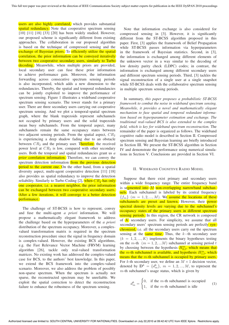Dn-1=[ 0 0 1 0 0 1 1 0 0 ] Dn =[ 1 0 1 0 0 1 0 0 0 ] frequency frequency As illustrated in Figure 2, we deﬁne a general correlation factor τ , which represents either the temporal or the spatial correlation level, which is given by τ 1 − Dn − Dn−1 M . (6) In section V, we will demonstrate that different correlation levels provide different performance gains. III. COMPRESSED SPECTRUM SENSING AND BAYESIAN LEARNING In this section, we brieﬂy introduce the compressed sensing and Bayesian learning, thus providing the background for our proposed ST-BCSS algorithm. A. Compressed Sensing Brieﬂy speaking, compressed sensing solves an ill-posed inverse problem. Given an N × 1 observation vector g and an N × M (N < M) matrix Φ, M × M matrix Ψ, the task is to ﬁnd an M × 1 solution vector f to satisfy an equation, which is given by g = ΦΨf , (7) where Φ is the compressed matrix and Ψ is the projection matrix. The vector f has a sparse representation projected by Ψ. When matrix Φ,Ψ and vector f satisfy the Restricted Isometry Property (RIP) [6], it can be solved by following optimization problem: ˜f = arg min˜f1 s.t. g = ΦΨ˜f . (8) Compressed sensing based Analog-to-Information Conver- sion (AIC) was proposed in [14] [21]. Eldar proposed a blind wideband analog reconstruction method [17]. Based on the autocorrelation reconstruction, [19] [30] [31] presented a scheme of analog signal acquisition, which endows us an implementation structure to acquire the wideband signal within an affordable hardware cost. In this paper, based on these implementation structures, we represent the analog signal acquisition in a projection matrix, for simplicity. We construct an N × M linear random sampling matrix A, to attain N time domain samples from discrete received signal yk, which is given by gk = Ayk + ˜nk, (9) where A can be a Gaussian or Bernoulli random matrix and the noise ˜nk remains to be white Gaussian noise. In wideband spectrum sensing, the vector yk can be represented sparsely in the Fourier transformation domain, which is given by yk = F−1wk, (10) where F−1 is the inverse Fourier transform matrix and wk is the sparse representation. Substituting (10) into (9) we obtain gk = AF−1wk + ˜nk = Θwk + ˜nk, (11) Fig. 2: An illustration of the spectrum temporal correlation where Θ = AF−1. Authorized licensed use limited to: SOUTH CENTRAL UNIVERSITY FOR NATIONALITIES. Downloaded on July 22,2010 at 09:42:42 UTC from IEEE Xplore. Restrictions apply.

This full text paper was peer reviewed at the direction of IEEE Communications Society subject matter experts for publication in the IEEE DySPAN 2010 proceedings B. Bayesian Learning In an iterative way, sm and qm can be update by λm, which To apply the Bayesian learning to recover the compressed signal [13] [32], the key idea is to establish a hierarchical prior. We assume that the noise upon the observations among cooperative secondary users are independent and identically distributed (i.i.d.), which is formulated as the following equa- tions (for notational simplicity we drop the secondary user’s label here): p(w|λ) = N (wi|0, λ−1 i ). (12) M i=1 First, we set up a zero-mean Gaussian prior on each element wi, which is satisﬁed a Normal distribution with zero mean and variance λ−1 . And we deﬁne the a posteriori probability for g, which is given by p(g|w, σ2) = (2πσ2) − g − Θw2 2 exp (13) − N . i 2σ2 And the posterior for w, given g, λ, and σ2 is the convolution of Gaussian random variables [25]: p(w|g, λ, σ2) = |Σ|− 1 − N+1 2 p(g|w, σ2)p(w|λ) p(g|λ, σ2) − 1 2 −1( ¯W) 2 exp = (2π) ,(14) where (•)H represents the vector or matrix conjugate trans- pose, and ( ¯W)HΣ ¯W = w − μ Σ = (σ−2ΘHΘ + Λ) μ = σ−2ΣΘHg. −1 With Λ = diag(λ1, λ2, ..., λM ), the goal of BCS is to attain the a posteriori mean μM P . An analytically tractable way to solve this problem is to maximization the logarithm of L(λ), which is given by L(λ) = log p(g|λ, σ2) ∞ p(g|w, σ2)p(w|λ)dw −∞ [N log 2π + log |C| + gHC −1g], = log = −1 2 with C = σ2I + ΘΛ −1ΘH , where I is the unit matrix. An efﬁcient algorithm to ﬁnd a λ that maximizes (18) is the Fast Marginal Likelihood Max- imization (FMLM) [9] [26]. The original FMLM deals with real-valued signals and measurement matrices. We derive the complex-valued FMLM in Appendix . [26] deﬁned ‘sparsity factor’ si and the ‘quality factor’ qi for each column θi in matrix Θ (the detailed deﬁnitions are omitted here). And λi can be updated using |si|2 |qi|2 − si λi = λi = ∞, , if|qi|2 > |si| if|qi|2 ≤ |si| (21) (15) (16) (17) (18) (19) (20) (22) (24) (25) (26) (27) is given by sm = λmSm λm − Sm λmQm λm − Sm qm = (23) when λm = ∞, sm = Sm and qm = Qm. Moreover, Sm and Qm can be easily obtained from , Sm = θH Qm = θH mBθm − θH mBg − θH mPTPH θm mPTPHg. where we deﬁne B = σ−2I PTPH = BΘΣΘHB. P is a unitary matrix (PPH = I) and T is a diagonal matrix with real-valued elements. Therefore, we can set up an initial λ and then attain S and Q. λ can also be update iteratively. When it converges, μMP can be attained from (17), as well as w = μMP. IV. SPACE-TIME BAYESIAN COMPRESSED SENSING the hierarchical prior In this section, we propose the novel ST-BCSS algorithm. in the original BCS is Note that non-informative. Since we can attain either temporal or spatial redundancy from previous detection results or from other cooperative secondary users, we can convey these information through the prior parameters. In this section, we address how to represent, convey, and fuse multiple a priori information sources. We assume that the compressed matrices are identical for all cooperative secondary users, which can be implemented by using the same random seed to generate the projection matrix. A. Representing the Prior Information In ST-BCSS, prior information can be exchanged between multi-prior entities. Firstly, we present a two-prior-entity sce- nario and then extend to multi-prior scenarios. 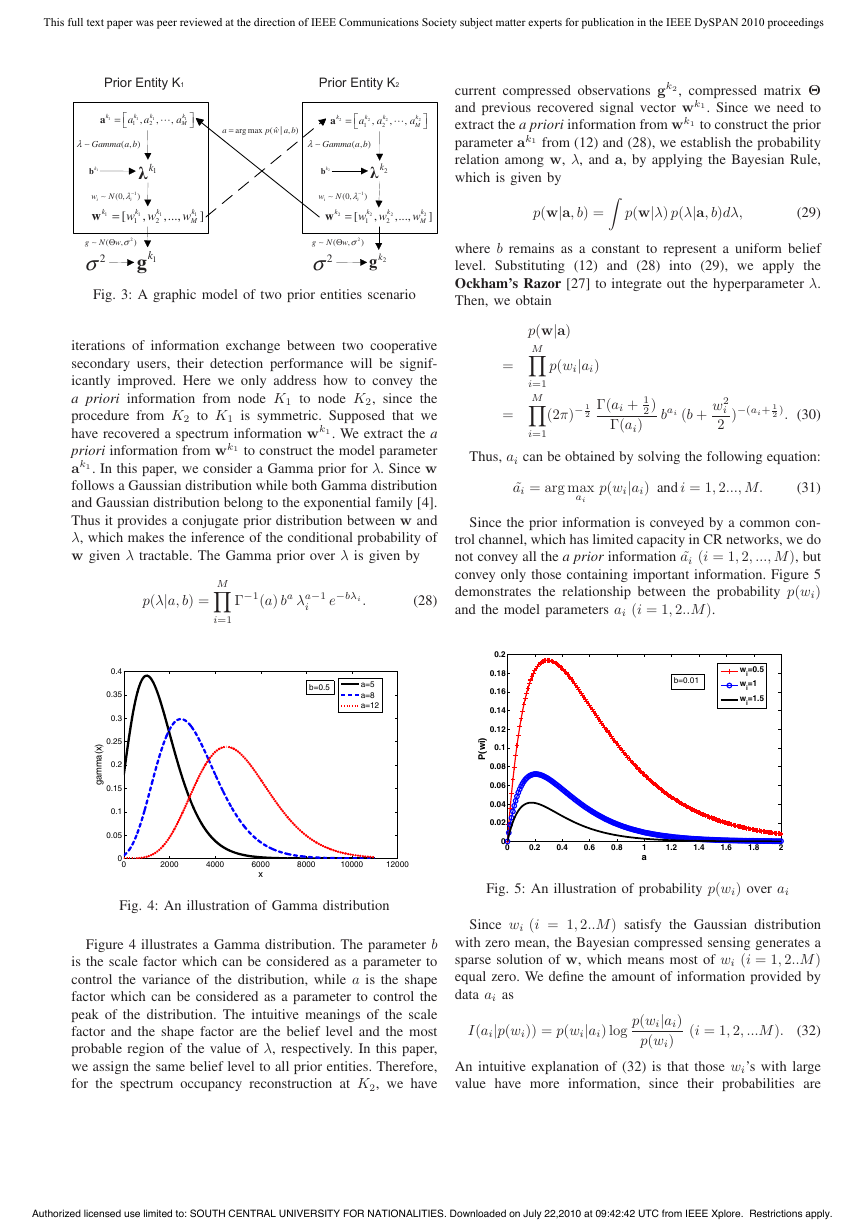We use a directed graph to illustrate the probabilistic model for each secondary user, as shown in Figure 3. Suppose that we have recovered two spectrum information entities, wk1 and wk2, from the compressed observation gk1 and gk2, respectively. From the temporal aspect, the prior information is conveyed from K1 to K2 as represented by the dash arrow, it is single direction information transportation. From the spatial aspect, the prior information is exchanged between K1 and K2, represented by the dash and solid arrows. Moreover, when a secondary user has only one collaborator, we can exchange the a priori information iteratively which is similar to Turbo decoding. This is especially useful when the capacity of control channel is limited and the secondary user is currently suffering a deep fading detection environ- ment. Our numerical simulation demonstrates that, after a few Authorized licensed use limited to: SOUTH CENTRAL UNIVERSITY FOR NATIONALITIES. Downloaded on July 22,2010 at 09:42:42 UTC from IEEE Xplore. Restrictions apply.

This full text paper was peer reviewed at the direction of IEEE Communications Society subject matter experts for publication in the IEEE DySPAN 2010 proceedings Prior Entity K1 Prior Entity K2 = k 1 a ⎡ ⎣ k a a 1 1 , k 1 2 , , a k 1 M ⎤ ⎦ λ∼ ( , ) Gamma a b = a arg max ( , ) p w a b | ˆ k 2 a = ⎡ ⎣ 2 k a 1 , 2 k a 2 , , a k 2 M ⎤ ⎦ λ∼ ( , ) Gamma a b 1kλ ) 1kb 1 i (0, w N λ− ∼ =w [ k 1 i k w w 1 2 k 1 1 , ,..., k w 1 M ] 2kλ ) 2kb 1 i w N λ− ∼ (0, =w [ k 2 i current compressed observations gk2, compressed matrix Θ and previous recovered signal vector wk1. Since we need to extract the a priori information from wk1 to construct the prior parameter ak1 from (12) and (28), we establish the probability relation among w, λ, and a, by applying the Bayesian Rule, which is given by 2 ,..., k w 2 M ] p(w|a, b) = k w w 2 k 1 , 2 p(w|λ) p(λ|a, b)dλ, (29) 2 , ( g N w σΘ∼ 2σ ) 1kg 2 , ( g N w σΘ∼ 2σ ) 2kg Fig. 3: A graphic model of two prior entities scenario where b remains as a constant to represent a uniform belief level. Substituting (12) and (28) into (29), we apply the Ockham’s Razor [27] to integrate out the hyperparameter λ. Then, we obtain iterations of information exchange between two cooperative secondary users, their detection performance will be signif- icantly improved. Here we only address how to convey the a priori information from node K1 to node K2, since the procedure from K2 to K1 is symmetric. Supposed that we have recovered a spectrum information wk1. We extract the a priori information from wk1 to construct the model parameter ak1. In this paper, we consider a Gamma prior for λ. Since w follows a Gaussian distribution while both Gamma distribution and Gaussian distribution belong to the exponential family [4]. Thus it provides a conjugate prior distribution between w and λ, which makes the inference of the conditional probability of w given λ tractable. The Gamma prior over λ is given by M −1(a) ba λa−1 i Γ e−bλi . 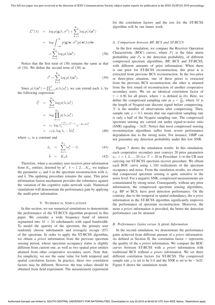(28) i=1 b=0.5 a=5 a=8 a=12 p(λ|a, b) = 0.4 0.35 0.3 0.25 0.2 0.15 0.1 0.05 ) x ( a m m a g 0 0 2000 4000 6000 x 8000 10000 12000 Fig. 4: An illustration of Gamma distribution Figure 4 illustrates a Gamma distribution. The parameter b is the scale factor which can be considered as a parameter to control the variance of the distribution, while a is the shape factor which can be considered as a parameter to control the peak of the distribution. The intuitive meanings of the scale factor and the shape factor are the belief level and the most probable region of the value of λ, respectively. In this paper, we assign the same belief level to all prior entities. Therefore, for the spectrum occupancy reconstruction at K2, we have p(wi|ai) p(w|a) M M i=1 i=1 − 1 2 (2π) Γ(ai + 1 2) Γ(ai) bai (b + w2 i 2 −(ai+ 1 ) 2 ). (30) = = Thus, ai can be obtained by solving the following equation: ˜ai = arg max ai p(wi|ai) and i = 1, 2..., M. 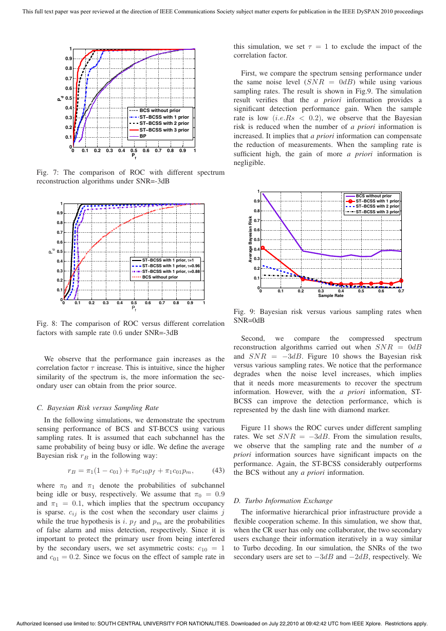(31) Since the prior information is conveyed by a common con- trol channel, which has limited capacity in CR networks, we do not convey all the a prior information ˜ai (i = 1, 2, ..., M), but convey only those containing important information. Figure 5 demonstrates the relationship between the probability p(wi) and the model parameters ai (i = 1, 2..M). b=0.01 wi=0.5 wi=1 wi=1.5 0.2 0.18 0.16 0.14 0.12 0.1 0.08 0.06 0.04 0.02 ) i w P ( 0 0 0.2 0.4 0.6 0.8 1.2 1.4 1.6 1.8 2 1 a Fig. 5: An illustration of probability p(wi) over ai Since wi (i = 1, 2..M) satisfy the Gaussian distribution with zero mean, the Bayesian compressed sensing generates a sparse solution of w, which means most of wi (i = 1, 2..M) equal zero. We deﬁne the amount of information provided by data ai as I(ai|p(wi)) = p(wi|ai) log (i = 1, 2, ...M). (32) p(wi|ai) p(wi) An intuitive explanation of (32) is that those wi’s with large value have more information, since their probabilities are Authorized licensed use limited to: SOUTH CENTRAL UNIVERSITY FOR NATIONALITIES. Downloaded on July 22,2010 at 09:42:42 UTC from IEEE Xplore. Restrictions apply.

This full text paper was peer reviewed at the direction of IEEE Communications Society subject matter experts for publication in the IEEE DySPAN 2010 proceedings small. Thus the corresponding ai’s offer more information. A good measure for the value of ai [4] is given by V (ai) = log p(wi|ai) − log p(wi) (33) according to the Therefore, channel condition, we apply (33) to select a certain number of ai (i ∈ U), where the set U contains T elements which are the indices of the chosen ai. common control information a, With the a priori the procedure of re- constructing the spectrum information is to ﬁnd a λ which maximizes the revised logarithm posterior likelihood. The revised logarithm posterior likelihood is given by L (λ) = log p(g|λ, σ2) + log p(λ|a) ∞ p(g|w, σ2)p(w|λ)dw + log p(λ|a) = log −∞ [N log 2π + log |C| + gHC = −1 T 2 (ai log λi − bλi). + −1g] (34) i=1 The derivatives of (34) with respect to log λi are given by ∂L ∂λi = si 2λi(λi + si) f(λi, si, qi, ai, b) − |qi|2 2(λi + si)2 + , − b ai λi = λi(λi + si)2 (35) where i ∈ U. To attain the optimal λi, we set l(λi) = 0. This is equivalent to solving the equation given by f(λi, si, qi, ai, b) = 0. (36) If current i ∈ U, we apply the revised λi update rule (the details of the updating procedure is given in Appendix ), which is given by λi = argλ {λ|f(λ, si, qi, ai, b) = 0} . (37) For those λi where i /∈ U, we apply (21) for updating the parameters. The procedure of spectrum occupancy reconstruction is summarized in procedure 1, as show below. B. Multi-prior Information Consequently, we extend the two-prior-entity processing to a multi-prior-entity one, which is illustrated in Figure 6. These priors are from both other cooperative secondary users and the previous recovered spectrum information. For the k-th secondary user with Kn prior entities, the reconstruction procedure is to ﬁnd a λ which maximizes the log likelihood L. Therefore, we rewrite (34) as Procedure 1 ST-BCSS compressed spectrum recover algo- rithm with priori information 1: Set λi with a initial value and j = 0 2: Sequentially compute the initial values: sm, qm, Σ, μ for 3: if j = Last Iteration then all M column vector θm 4: 5: 6: 7: 8: Select a candidate column vector θi from Θ and com- pute the indicator ηi |qi|2 − si if ηi > 0 & λi < ∞ then else if ηi > 0 & λi = ∞ then Re-estimate λi into the else if ηi ≤ 0 then Computeλi by solving (21) and add θi selected set Delete θi from selected set and set λi = ∞ end if Compute the log likelihood L(λ) if ΔL(λ) ≤ T hreshold then 9: 10: 11: 12: 13: 14: 15: 16: 17: 18: end if 19: Compute the prior ˜a by (31) 20: Apply (32), compute the information metrics for each j = LastIteration j = j + 1 end if else ˜ai, i = 1, 2, ..., M 21: Select the ˜ak, k = 1, 2, ..., T with T largest information metrics. 22: return return w and ˜ak Prior Entity K1 Prior Entity K2 k 1 a = ⎣ ⎡ k a a 1 1 , k 1 2 , , a k 1 M ⎤ ⎦ λ∼ ( , ) Gamma a b k 2 a = ⎡ ⎣ 2 k a 1 , 2 k a 2 , , a k 2 M ⎤ ⎦ λ∼ ( , ) Gamma a b 1kλ ) 1kb 1 i (0, w N λ− ∼ =w [ k 1 i k w w 1 2 k 1 1 , ,..., k w 1 M ] 2kλ ) 2kb 1 i w N λ− ∼ (0, =w [ k 2 i k w w 2 k 1 , 2 2 ,..., k w 2 M ] 2 , ( g N w σΘ∼ 2σ ) 1kg 2 , ( g N w σΘ∼ 2σ ) 2kg Prior Entity K3 = k 3 a k a 3 1 , k a 3 2 ⎡ ⎣ , , k a 3 M ⎤ ⎦ λ∼ ( , ) Gamma a b 3kb 3kλ Prior Entity K4 k 4 a = ⎡ ⎣ 4 k a 1 , 4 a k 2 , , a k 4 M ⎤ ⎦ λ∼ ( , ) Gamma a b 4kb 4kλ 1 i w N λ− ∼ (0, =w [ k 3 i ) k 3 1 k w w 2 , 3 ,..., k w 3 M ] i w N λ− ∼ (0, =w [ k 4 i 1 ) k k w w 1 2 , 4 4 ,..., k w 4 M ] 2 , ( g N w σΘ∼ 2σ ) 3kg 2 , ( g N w σΘ∼ 2σ ) 4kg Fig. 6: Multi-prior information exchange among cooperative secondary users Authorized licensed use limited to: SOUTH CENTRAL UNIVERSITY FOR NATIONALITIES. Downloaded on July 22,2010 at 09:42:42 UTC from IEEE Xplore. Restrictions apply.

This full text paper was peer reviewed at the direction of IEEE Communications Society subject matter experts for publication in the IEEE DySPAN 2010 proceedings L (λ) = log p(g|λ, σ2) + Kn k=1 log p(λ|ak) = log p(g|w, σ2)p(w|λ)dw −∞ log p(λ|ak). ∞ Kn + k=1 Kn log p(λ|ak). l 2 = k=1 T i=1 p(λi|ak Kn l 2 i = log p(λi|ak i ) Kn k=1 k=1 = log p(λi|ak i ) Kn i −1) k=1(ak = c1 log λ = c1˜ai log λi − ˜bλk i . i e−Knbλk i Notice that the ﬁrst term of (38) remains the same as that of (34). We deﬁne the second term of (38) as Since p(λ|ak) = the following expression: i ), we can extend each λi by (38) (39) (40) (41) (42) for the correlation factors and the test for the ST-BCSS algorithm will be our future work. A. Comparison between BP, BCS and ST-BCCS three-prior situation, one of In the ﬁrst simulation, we compare the Receiver Operation Characteristic (ROC) curves, where Pf is the false alarm probability and Pd is the detection probability, of different compressed spectrum algorithms, BP, BCS and ST-BCSS, with different amounts of prior information. When there this prior a is is one prior for ST-BCSS reconstruction, extracted from previous BCS reconstruction. In the two-prior or these priors is extracted from the previous BCS reconstruction, the other is attained from the ﬁrst round of reconstruction of another cooperative secondary users. We set an identical correlation factor of τ = 0.96 for all priors, where τ is deﬁned in (6). Here, we deﬁne the compressed sampling rate as ρ = N M , where M is the length of Nyquist-rate discrete signal before compressing, N is the number of observations after compressing. Then, sample rate ρ = 0.5 means that our equivalent sampling rate is only a half of the Nyquist sampling rate. The compressed spectrum sensing are carried out under signal-to-noise ratio (SNR) equaling −3dB. Notice that most compressed sensing reconstruction algorithms suffer from severe performance degradation due to the strong noise. For instance, OMP can not guarantee any detection probability under this low SNR. Figure 7 shows the simulation results. In this simulation, each cooperative secondary user conveys 20 prior parameters ai, i = 1, 2, ..., 20 (i.e. T = 20 in Procedure 1) to the CR user carrying out ST-BCSS spectrum recover procedure. We obtain each ROC curve using 1, 500 realizations of the spectrum occupancy and noise. From the simulation results, we observe that compressed spectrum sensing is quite sensitive to the noise level. For a negative SNR, compressed measurements are contaminated by strong noise. Consequently, without any prior information, the compressed spectrum sensing algorithms, e.g. BP or BCS, have poor detection performance. On the contrary, due to the temporal or spatial redundancy, the a prior information in the ST-BCSS algorithm signiﬁcantly improves the performance of spectrum reconstruction. Moreover, the more a priori information is provided, the better the detection performance can be attained. B. Performance Gains versus A priori Information In the second simulation, we demonstrate the performance gains achieved from different amount of a priori information. As deﬁned in Section II, the correlation factor τ represents the quality of the a priori information. We compare the ROC curves between ST-BCSS with a priori information with traditional BCS without a priori information. We set three different correlation factors for ST-BCSS. The compressed sample rate ρ is set to be 0.6 and the SNR is set to be −3dB. Figure 8 shows the simulation result. where c1 is a constant and ˜ai = Kn i − 1) (ak k=1 ˜b = Knb. Therefore, when a secondary user receives prior information from Kn entities, denoted by ak, k = 1, 2..., Kn, we replace the parameter ai and b in the spectrum reconstruction with ˜ai and ˜b. The updating procedure remains the same. This prior information fusion mechanism provides the robustness against the variation of the cognitive radio network scale. Numerical simulations will demonstrate the performance gain by applying the multi-prior information. V. NUMERICAL SIMULATIONS the sparsity of the spectrum, In this section, we use numerical simulations to demonstrate the performance of the ST-BCCS algorithm proposed in this paper. We consider a wide frequency band of interest segmented into M = 50 subchannels with equal bandwidth. To model the primary user randomly choose subchannels and averagely occupy 20% of the spectrum. In order to apply the ST-BCSS algorithm, we obtain a priori information from the previous spectrum sensing period, whose spectrum occupancy status is slightly different from current one, as well as two spatial prior entities attained from other cooperative secondary users. Note that, for simplicity, we use the same value for both temporal and spatial correlation factors. In practice, these two correlation factors may be different. However, the true values should be obtained from ﬁeld experiment. The measurement experiment Authorized licensed use limited to: SOUTH CENTRAL UNIVERSITY FOR NATIONALITIES. Downloaded on July 22,2010 at 09:42:42 UTC from IEEE Xplore. Restrictions apply.

This full text paper was peer reviewed at the direction of IEEE Communications Society subject matter experts for publication in the IEEE DySPAN 2010 proceedings 1 0.9 0.8 0.7 0.6 d P 0.5 0.4 0.3 0.2 0.1 0 0 this simulation, we set τ = 1 to exclude the impact of the correlation factor. BCS without prior ST−BCSS with 1 prior ST−BCSS with 2 prior ST−BCSS with 3 prior BP 0.1 0.2 0.3 0.4 0.5 P f 0.6 0.7 0.8 0.9 1 the a priori First, we compare the spectrum sensing performance under the same noise level (SN R = 0dB) while using various sampling rates. The result is shown in Fig.9. The simulation result veriﬁes that information provides a signiﬁcant detection performance gain. When the sample rate is low (i.e.Rs < 0.2), we observe that the Bayesian risk is reduced when the number of a priori information is increased. It implies that a priori information can compensate the reduction of measurements. When the sampling rate is sufﬁcient high, information is negligible. the gain of more a priori Fig. 7: The comparison of ROC with different spectrum reconstruction algorithms under SNR=-3dB 1 0.9 0.8 0.7 0.6 d P 0.5 0.4 0.3 0.2 0.1 0 0 ST−BCSS with 1 prior, τ=1 ST−BCSS with 1 prior, τ=0.96 ST−BCSS with 1 prior, τ=0.88 BCS without prior 0.1 0.2 0.3 0.4 0.5 P f 0.6 0.7 0.8 0.9 1 Fig. 8: The comparison of ROC versus different correlation factors with sample rate 0.6 under SNR=-3dB We observe that the performance gain increases as the correlation factor τ increase. This is intuitive, since the higher similarity of the spectrum is, the more information the sec- ondary user can obtain from the prior source. C. Bayesian Risk versus Sampling Rate In the following simulations, we demonstrate the spectrum sensing performance of BCS and ST-BCCS using various sampling rates. It is assumed that each subchannel has the same probability of being busy or idle. We deﬁne the average Bayesian risk rB in the following way: rB = π1(1 − c01) + π0c10pf + π1c01pm, (43) where π0 and π1 denote the probabilities of subchannel being idle or busy, respectively. We assume that π0 = 0.9 and π1 = 0.1, which implies that the spectrum occupancy is sparse. cij is the cost when the secondary user claims j while the true hypothesis is i. pf and pm are the probabilities of false alarm and miss detection, respectively. Since it is important to protect the primary user from being interfered by the secondary users, we set asymmetric costs: c10 = 1 and c01 = 0.2. Since we focus on the effect of sample rate in BCS without prior ST−BCSS with 1 prior ST−BCSS with 2 prior ST−BCSS with 3 prior 1 0.9 0.8 0.7 0.6 0.5 0.4 0.3 0.2 0.1 i i k s R n a s e y a B e g a r e v A 0 0 0.1 0.2 0.3 0.4 Sample Rate 0.5 0.6 0.7 Fig. 9: Bayesian risk versus various sampling rates when SNR=0dB the compare compressed Second, we spectrum reconstruction algorithms carried out when SN R = 0dB and SN R = −3dB. Figure 10 shows the Bayesian risk versus various sampling rates. We notice that the performance degrades when the noise level increases, which implies it needs more measurements to recover the spectrum that information. However, with the a priori information, ST- BCSS can improve the detection performance, which is represented by the dash line with diamond marker. Figure 11 shows the ROC curves under different sampling rates. We set SN R = −3dB. From the simulation results, we observe that the sampling rate and the number of a priori information sources have signiﬁcant impacts on the performance. Again, the ST-BCSS considerably outperforms the BCS without any a priori information. D. Turbo Information Exchange The informative hierarchical prior infrastructure provide a ﬂexible cooperation scheme. In this simulation, we show that, when the CR user has only one collaborator, the two secondary users exchange their information iteratively in a way similar to Turbo decoding. In our simulation, the SNRs of the two secondary users are set to −3dB and −2dB, respectively. We Authorized licensed use limited to: SOUTH CENTRAL UNIVERSITY FOR NATIONALITIES. Downloaded on July 22,2010 at 09:42:42 UTC from IEEE Xplore. Restrictions apply.

分享到：

赞收藏

资料库

贝叶斯压缩感知算法.pdf

相关推荐

课程资源

热门标签

最新资料