Recent Progresses in Deep Learning based Acoustic
Models (Updated)
Dong Yu and Jinyu Li
Tencent AI Lab, USA., Microsoft AI and Research, USA.
dongyu@ieee.org, jinyli@microsoft.com
1
8
1
0
2
r
p
A
7
2
]
S
A
.
s
s
e
e
[
2
v
8
9
2
9
0
.
4
0
8
1
:
v
i
X
r
a
Abstract—In this paper, we summarize recent progresses made
in deep learning based acoustic models and the motivation and
insights behind the surveyed techniques. We first discuss acoustic
models that can effectively exploit variable-length contextual
information, such as recurrent neural networks (RNNs), convo-
lutional neural networks (CNNs), and their various combination
with other models. We then describe acoustic models that are
optimized end-to-end with emphasis on feature representations
learned jointly with rest of the system, the connectionist temporal
classification (CTC) criterion, and the attention-based sequence-
to-sequence model. We further illustrate robustness issues in
speech recognition systems, and discuss acoustic model adapta-
tion, speech enhancement and separation, and robust training
strategies. We also cover modeling techniques that
lead to
more efficient decoding and discuss possible future directions
in acoustic model research. 1
Index Terms—Speech Processing, Deep Learning, LSTM,
CNN, Speech Recognition, Speech Separation, Permutation In-
variant Training, End-to-End, CTC, Attention Model, Speech
Adaptation
I. INTRODUCTION
In the past several years, there has been significant progress
in automatic speech recognition (ASR) [1]–[21]. These pro-
gresses have led to ASR systems that surpassed the threshold
for adoption in many real-world scenarios and enabled services
such as Google Now, Microsoft Cortana, and Amazon Alexa.
Many of these achievements are powered by deep learning
(DL) techniques. Readers are referred to Yu and Deng 2014
[22] for a comprehensive summary and detailed description of
the technology advancements in ASR made before 2015.
In this paper, we survey new developments happened in
the past two years with an emphasis on acoustic models. We
discuss motivations behind, and core ideas of, each interesting
work surveyed. More specifically, in Section II we illustrate
improved DL/HMM hybrid acoustic models that employ deep
recurrent neural networks (RNNs) and deep convolutional
neural networks (CNNs). These hybrid models can better
exploit contextual
information than deep neural networks
(DNNs) and thus lead to new state-of-the-art recognition
accuracy. In Section III we describe acoustic models that
are designed and optimized end-to-end with no or less non-
learn-able components. We first discuss the models in which
audio waveforms are directly used as the input feature so
1This is an updated version with latest literature until ICASSP2018 of the
paper: Dong Yu and Jinyu Li, “Recent Progresses in Deep Learning based
Acoustic Models,” vol.4, no.3, IEEE/CAA Journal of Automatica Sinica,
2017.
that the feature representation layer is automatically learned
instead of manually designed. We then depict models that
are optimized using the connectionist temporal classification
(CTC) criterion which allows for a sequence-to-sequence
direct optimization. Following that we analyze models that
are built using attention-based sequence-to-sequence model.
We devote Section IV to discuss techniques that can improve
robustness with focuses on adaptation techniques, speech
enhancement and separation techniques, and robust training. In
Section V we describe acoustic models that support efficient
decoding techniques such as frame-skipping, teacher-student
training based model compression, and quantization during
training. We propose core problems to work on and potential
future directions in solving them in Section VI.
II. ACOUSTIC MODELS EXPLOITING VARIABLE-LENGTH
CONTEXTUAL INFORMATION
The DL/HMM hybrid model [1]–[5] is the first deep
learning architecture that succeeded in ASR and is still the
dominant model used in industry. Several years ago, most
hybrid systems are DNN based. As reported in [3], one of
the important factors that lead to superior performance in the
DNN/HMM hybrid system is its ability to exploit contextual
information. In most systems, a window of 9 to 13 frames
(left/right context of 4-6 frames) of features are used as the
input to the DNN system to exploit the information from
neighboring frames to improve the accuracy.
However, the optimal length of contextual information may
vary for different phones and speaking speed. This indicates
that using fixed-length context window, as in the DNN/HMM
hybrid system, may not be the best choice to exploit contextual
information. In recent years people have proposed new models
that can exploit variable-length contextual information more
effectively. The most important two models use deep RNNs
and CNNs.
A. Recurrent Neural Networks
Feed-forward DNNs only consider information in a fixed-
length sliding window of frames and thus cannot exploit long-
range correlations in the speech signal. On the other hand,
RNNs can encode sequence history in their internal states,
and thus have the potential to predict phonemes based on all
the speech features observed up to the current frame. Unfor-
tunately, simple RNNs, depending on the largest eigenvalue
of the state-update matrix, may have gradients which either
�
increase or decrease exponentially over time. Hence, the basic
RNNs are difficult to train, and in practice can only model
short-range effects.
Long short-term memory (LSTM) RNNs [23] were devel-
oped to overcome these problems. LSTM-RNNs use input,
output and forget gates to control information flow so that
gradients can be propagated in a stable fashion over relatively
longer span of time. These networks have been shown to
outperform DNNs on a variety of ASR tasks [8], [24]–[27].
Note that there is another popular RNN model, called gated
recurrent unit (GRU), which is simpler than LSTM but is also
able to model the long short-term correlation. Although GRU
has been shown effective in several machine learning tasks
[28], it is not widely used in ASR tasks.
At the time step t, the vector formulas of the computation
of LSTM units can be described as:
it = σ(Wixxt + Wihht−1 + pi ct−1 + bi)
ft = σ(Wf xxt + Wf hht−1 + pf ct−1 + bf )
ct = ft ct−1 + it φ(Wcxxt + Wchht−1 + bc)
ot = σ(Woxxt + Wohht−1 + po ct + bo)
ht = ot φ(ct)
(1a)
(1b)
(1c)
(1d)
(1e)
where xt is the input vector. The vectors it, ot, ft are the
activation of the input, output, and forget gates, respectively.
The W.x and W.h terms are the weight matrices for the inputs
xt and the recurrent inputs ht−1, respectively. The pi, po, pf
are parameter vectors associated with peephole connections.
The functions σ and φ are the logistic sigmoid and hyperbolic
tangent nonlinearity, respectively. The operation represents
element-wise multiplication of vectors.
It is popular to stack LSTM layers to get better modeling
power [8]. However, an LSTM-RNN with too many vanilla
LSTM layers is very hard to train and there still exists the
gradient vanishing issue if the network goes too deep. This
issue can be solved by using either highway LSTM or residual
LSTM.
In the highway LSTM [29], memory cells of adjacent layers
are connected by gated direct links which provide a path
for information to flow between layers more directly without
decay. Therefore, it alleviates the gradient vanishing issue and
enables the training of much deeper LSTM-RNN networks.
Residual LSTM [30], [31] uses shortcut connections be-
tween LSTM layers, and hence also provides a way to allevi-
ating the gradient vanishing problem. Different from highway
LSTM which uses gates to guide the information flow, residual
LSTM is more straightforward with the direct shortcut path,
similar to Residual CNN [32] which recently achieves great
success in the image classification task.
Typically, log Mel-filter-bank features are often used as the
input to the neural-network-based acoustic model [33], [34].
Switching two filter-bank bins will not affect the performance
of the DNN or LSTM. However, this is not the case when a
human reads a spectrogram: a human relies on both patterns
that evolve over time and frequency to predict phonemes. This
inspired the proposal of a 2-D, time-frequency (TF) LSTM
[35]–[37] which jointly scans the speech input over the time
and frequency axes to model spectro-temporal warping, and
2
then uses the output activations as the input to the traditional
time LSTM. The joint
time-frequency modeling provides
better normalized features for the upper layer time LSTMs.
This has been verified effective and robust to distortion at
both Microsoft and Google on large-scale tasks (e.g., Google
home [38]). Note that the 2D-LSTM processes along time and
frequency axis sequentially, hence it increases computational
complexity. In [39], several solutions have been proposed to
reduce the computational cost.
Highway LSTM has gates on both the temporal and spatial
directions while TF LSTM has gates on both the temporal and
spectral directions. It is desirable to have a general LSTM
structure that works along all directions. Grid LSTM [40]
is such a general LSTM which arranges the LSTM memory
cells into a multidimensional grid. It can be considered as
a unified way of using LSTM for temporal, spectral, and
spatial computation. Grid LSTM has been studied for temporal
and spatial computation in [41] and temporal and spectral
computation in [37].
Although bi-directional LSTMs (BLSTMs) perform better
than uni-directional LSTMs by using the past and future
context information [8], [42], they are not suitable for real-time
systems since the recognition can happen only after the whole
utterance has been observed. For this reason, models, such
as latency-controlled BLSTM (LC-BLSTM) [29] and row-
convolution BLSTM (RC-BLSTM), that bridge between uni-
directional LSTMs and BLSTMs have been proposed. In these
models, the forward LSTM is still kept as is. However, the
backward LSTM is replaced by either a backward LSTM with
at most N-frames of lookahead as in the LC-BLSTM case,
or a row-convolution operation that integrates information in
the N-frames of lookahead. By carefully choosing N we can
balance between recognition accuracy and latency. Recently,
LC-BLSTM was improved by [43] to speed up the evaluation
and to enable real-time online speech recognition by using
better network topology to initialize the BLSTM memory cell
states.
B. Convolutional Neural Networks
Another model that can effectively exploit variable-length
contextual information is the convolutional neural network
(CNN) [44], in the center of which is the convolution operation
(or layer). The input to the convolution operation is usually
a three-dimensional tensor (row, column, channel) for speech
recognition but can be lower or higher dimensional tensors for
other applications. Each channel of the input and output of the
convolution operation can be considered as a view of the same
data. In most setups, all channels have the same size (height,
width).
The filters in the convolution operation are called kernels,
tensors (kernel height, kernel
which are four-dimensional
width, input channel, output channel) in our case. There are
in total Cx × Cv kernels, where Cx is the number of input
channels and Cv is the number of output channels. The kernels
are applied to local regions called receptive fields in an input
�
image along all channels. The value after the convolution
operation is
υij (K, X) =
vec (Kn) · vec (Xijn) ,
(2)
n
for each output channel and input slice (i, j) (the i-th step
along the vertical direction and j-th step along the horizontal
direction), where Kn of size (Hk, Wk) is a kernel matrix
associated with input channel n and output channel and has
the same size as the input image patch Xijn of channel n,
vec(˙) is the vector formed by stacking all the columns of the
matrix, and · is the inner product of two vectors. It is obvious
that each output pixel is a weighted sum of all pixels across
all channels in an input patch. Since each input pixel can be
considered as a weak patten detector, each output pixel is just a
boosted detector exploiting all information in the input patch.
The kernel is shared across all input patches and moves
along the input image with strides Sr and Sc at the vertical
and horizontal direction, respectively. When the strides are
larger than 1, the convolution operation also subsamples, in
additional to convolving, the input image and leads to a lower-
resolution image that is less sensitive to the small pattern shift
inside the input patch. The translational invariance can be fur-
ther improved when some kind of aggregation operations are
applied after the convolution operation. Typical aggregation
operations are max-pooling and average-pooling. The aggrega-
tion operations often go with subsampling to reduce resolution.
Due to the built-in translational invariability CNNs can exploit
variable-length contextual information along both frequency
and time axes. It is obvious that if only one convolution layer
is used the translational variability the system can tolerate
is limited. To allow for more powerful exploitation of the
variable-length contextual information, convolution operations
(or layers) can be stacked.
The time delay neural network (TDNN) [45] was the first
model that exploits multiple CNN layers for ASR. In this
model, convolution operations are applied to both time and
frequency axes. However, the early TDNNs are neural network
only solution that do not integrate with HMMs and are hard
to be used in large vocabulary continuous speech recognition
(LVCSR).
After the successful application of DNNs to LVCSR, CNNs
were reintroduced under the DL/HMM hybrid model architec-
ture [5], [7], [11], [14], [17], [46], [47], [47], [48]. Because
HMMs in the hybrid model already have strong ability to
handle variable-length utterance problem in ASR, CNNs were
reintroduced initially to deal with variability at the frequency
axis only [5], [7], [46], [47]. The goal was to improve robust-
ness against vocal tract length variability between different
speakers. Only one to two CNN layers were used in these early
models, stacked with additional fully-connected DNN layers.
These models have shown around 5% relative recognition error
rate reduction compared to the DNN/HMM systems [7]. Later,
additional RNN layers, e.g., LSTMs, were integrated into the
model to form so called CNN-LSTMM-DNN (CLDNN) [10]
and CNN-DNN-LSTM (CDL) architectures. The RNNs in
these models can help to exploit the variable-length contextual
information since CNNs in these models only deal with
3
frequency-axis variability. CLDNN and CDL both achieved
additional accuracy improvement over CNN-DNN models.
information, attracted new attentions,
Researchers quickly realized that dealing with variable-
length utterance is different from exploiting variable-length
contextual information. TDNNs, which convolve along both
the frequency and time axes and thus exploit variable-length
contextual
this time
under the DL/HMM hybrid architecture [13], [49] and with
variations such as row convolution [15] and feedforward se-
quential memory network (FSMN) [16]. Similar to the original
TDNNs, these models stack several CNN layers along the
frequency and time-axis, with a focus on the time-axis, to
account for speaking rate variation. But unlike the original
TDNNs, the TDNN/HMM hybrid systems can recognize large
vocabulary continuous speech very effectively.
More recently, primarily motivated by the successes in
image recognition, various architectures of deep CNNs [14],
[17], [48], [50] have been proposed and evaluated for ASR.
The premise is that spectrograms can be seen as images
with special patterns from which experienced people can tell
what has been said. In deep CNNs, each higher layer is a
weighted sum of nonlinear transformation of a window of
lower layers and thus covers longer contexts and operates on
more abstract patterns. Lower CNN layers capture local simple
patterns while higher CNN layers detect broader, abstract,
and more complicated patterns. Smaller kernels combined
with more layers allow deep CNNs to exploit longer-range
dependency information along both time and frequency axes
more effectively. Empirically deep CNNs are compatible
to BLSTMs [19], which in turn outperform unidirectional
LSTMs. However, unlike BLSTMs which suffer from long
latency, because you need to wait for the whole utterance to
finish to start decoding, and cannot be deployed in real-time
systems, deep CNNs have limited latency and are better suited
for real-time systems if the computation cost can be controlled.
Training and evaluation of deep CNNs is very time consum-
ing, esp. if we treat each window of frames independently,
under which condition there are significant duplication of
computations. To speedup the computation we can treat the
whole utterance as a single input image and thus reuse the
intermediate computation results. Even better,
if the deep
CNN is designed so that the stride at each layer is long
enough to cover the whole kernel, similar to the CNNs with
layer-wise context expansion and attention (LACE) [17]. Such
model, called dilated CNN [48], allows to exploit longer-range
information with less number of layers and can significantly
reduce the computational cost. Dilated CNN has outperformed
other deep CNN models on the switchboard task [48].
Note that deep CNNs can be used together with RNNs and
under frameworks such as connectionist temporal classification
(CTC) that we will discuss in Section III-B.
III. ACOUSTIC MODELS WITH END-TO-END
OPTIMIZATION
The models discussed in the previous
section are
DNN/HMM hybrid models in which the two components
DNN and HMM are usually optimized separately. However,
�
speech recognition is a sequential recognition problem. It is
not surprising that better recognition accuracy may be achieved
if all components in a model are jointly optimized. Even better,
if the model can remove all manually designed components
such as basic feature representation and lexicon design.
was reduced by converting the time-domain convolution into
the frequency-domain product [61]. Later,
the CNN layer
was replaced by the 2D-LSTM layer [37] to improve the
robustness, and Google home was built with this end-to-end
system [38].
A. Automatically Learned Audio Feature Representation
B. Connectionist Temporal Classification
4
It is always arguable that the manually-designed log Mel-
filter-bank feature is optimal for speech recognition. Inspired
by the end-to-end processing in the machine learning commu-
nity, there are always efforts [51]–[54] trying to replace the
Mel-filter-bank extraction by directly learning filters using a
network to process the raw speech waveforms and training
it jointly with the recognizer network. Among these efforts,
the CLDNN [10] on raw waveform work [54] seems to be
more promising as it got slight gain over the log Mel-filter-
bank feature while the other works didn’t. More importantly, it
serves a good foundation of the multichannel processing with
raw waveforms.
The most critical thing for raw waveform processing is
using a representation that is invariant to small phase shift
because the raw waveforms are perceptually identical if the
only difference is a small phase shift. To achieve the phase
invariance, a time convolutional layer is applied to the raw
waveform and then pooling is done over the entire time length
of the time-convolved output signal. This process reduces the
temporal variation (hence phase invariant) and is very similar
to the Gammatone filterbank extraction. The pooled outputs
can be considered as the filter-bank outputs, on which the
standard CLDNN [10] is applied. Interestingly, the same idea
was recently applied to anti-spoofing speaker verification task
with significant gain [55].
With the application of deep learning models, now the
ASR systems on close-talking scenario perform very well. The
research interest is shifted to the far-field ASR which needs
to handle both additive noise and reverberation. The current
dominant approach is still using the traditional beamforming
method to process the waveforms from multiple microphones,
and then inputting the beamformed signal into the acoustic
model [56]. Efforts have also been made to use deep learning
models to perform beamforming and to jointly train the
beamforming and recognizer networks [57]–[60]. In [57], the
beamforming network and recognizer networks were trained
in a sequence by first training the beamforming network, then
training the recognizer network with the beamformed signal,
and finally jointly training both networks.
In [58]–[60], both networks were jointly trained in a more
end-to-end fashion by extending the aforementioned CLDNN
to raw waveform. In the first layer, multiple time convolution
filters are used to map the raw waveforms from multiple
microphones into a single time-frequency representation [58].
Then the output is passed to the upper layer CLDNN for
phoneme classification. Later, the joint network is improved by
factorizing the spatial and spectral selectivity of bottom layer
network into a spatial filtering layer and a spectral filtering
layer. The factored network brings accuracy improvement
with the cost of increasing computational cost, which later
Speech recognition task is a sequence-to-sequence task,
which maps the input waveform to a final word sequence or an
intermediate phoneme sequence. What the acoustic modeling
cares is the output of word or phoneme sequence, instead
of the frame-by-frame labeling which the traditional cross
entropy (CE) training criterion cares. Hence, the Connectionist
Temporal Classification (CTC) approach [9], [62], [63] was
introduced to map the speech input frames into an output label
sequence. As the number of output labels is smaller than that
of input speech frames, CTC path is introduced to force the
output to have the same length as the input speech frames by
adding blank as an additional label and allowing repetition of
labels.
Denote x as the speech input sequence, l as the original
label sequence, and B−1(l) represents all
the CTC paths
mapped from l. Then, the CTC loss function is defined as
the sum of negative log probabilities of correct labels as
(3)
(4)
T
LCT C = −lnP (l|x),
where
P (l|x) =
P (z|x)
z∈B−1(l)
With the conditional independent assumption, P (z|x) can be
decomposed into a product of posterior from each frame as
P (z|x) =
P (zt|x).
(5)
t=1
In [62], CTC with context-dependent phone output units
have been shown to outperform CTC with monophone [9], and
to perform in par with the LSTM model with cross entropy
criterion when training data is large enough. One attractive
characteristics of CTC is that because the output unit is usually
phoneme or unit larger than phoneme, it can take larger input
time step instead of single 10ms frame shift. For example, in
[62], three 10ms frames are stacked together as the input to
CTC models. By doing so, the acoustic score evaluation and
decoding happen every 30ms, 3 times faster than the traditional
systems that operate on 10ms frame shift.
The most attractive characteristics of CTC is that it provides
a path to end-to-end optimization of acoustic models. In the
deep speech [15], [64] and EESEN [65], [66] work, the end-to-
end speech recognition system is explored to directly predict
characters instead of phonemes, hence removing the need of
using lexicons and decision trees which are the building blocks
in [9], [62], [63]. This is one step toward removing expert
knowledge when building an ASR system. Another advantage
of character-based CTC is that it is more robust to the accented
speech as the graphoneme sequence of words is less affected
by accents than the phoneme pronunciation [67]. Other output
�
units that are larger than characters but smaller than words
have also been studied [68].
It
is a design challenge to determine the basic output
unit to use for CTC prediction. In all the aforementioned
works, the decomposition of a target word sequence into a
sequence of basic units is fixed. However, the pre-determined
fixed decomposition is not necessarily optimal. In [69], gram-
CTC was proposed to automatically learn the most suitable
decomposition of target sequences. Gram-CTC is based on
characters, but allows to output variable number of characters
(i.e., gram) at each time step. This not only boosts the
modeling flexibility but also improves the final ASR system
accuracy.
As the goal of ASR is to generate a word sequence from the
speech waveform, word unit is the most natural output unit for
network modeling. In [62], CTC with word output targets was
explored but the accuracy is far from the phoneme-based CTC
system. In [18], it was shown that by using 100k words as the
output targets and by training the model with 125k hours of
data, the CTC system with word units can beat the CTC system
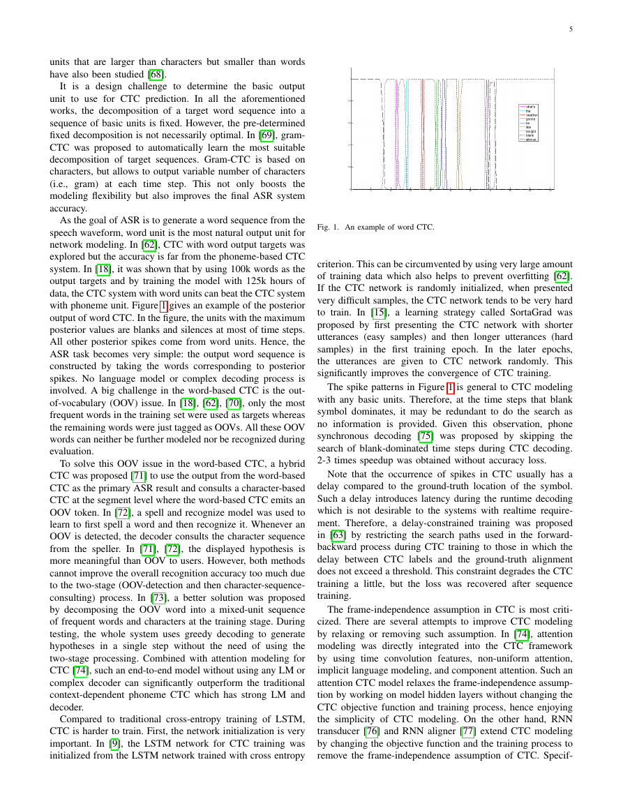
with phoneme unit. Figure 1 gives an example of the posterior
output of word CTC. In the figure, the units with the maximum
posterior values are blanks and silences at most of time steps.
All other posterior spikes come from word units. Hence, the
ASR task becomes very simple: the output word sequence is
constructed by taking the words corresponding to posterior
spikes. No language model or complex decoding process is
involved. A big challenge in the word-based CTC is the out-
of-vocabulary (OOV) issue. In [18], [62], [70], only the most
frequent words in the training set were used as targets whereas
the remaining words were just tagged as OOVs. All these OOV
words can neither be further modeled nor be recognized during
evaluation.
To solve this OOV issue in the word-based CTC, a hybrid
CTC was proposed [71] to use the output from the word-based
CTC as the primary ASR result and consults a character-based
CTC at the segment level where the word-based CTC emits an
OOV token. In [72], a spell and recognize model was used to
learn to first spell a word and then recognize it. Whenever an
OOV is detected, the decoder consults the character sequence
from the speller. In [71], [72], the displayed hypothesis is
more meaningful than OOV to users. However, both methods
cannot improve the overall recognition accuracy too much due
to the two-stage (OOV-detection and then character-sequence-
consulting) process. In [73], a better solution was proposed
by decomposing the OOV word into a mixed-unit sequence
of frequent words and characters at the training stage. During
testing, the whole system uses greedy decoding to generate
hypotheses in a single step without the need of using the
two-stage processing. Combined with attention modeling for
CTC [74], such an end-to-end model without using any LM or
complex decoder can significantly outperform the traditional
context-dependent phoneme CTC which has strong LM and
decoder.
Compared to traditional cross-entropy training of LSTM,
CTC is harder to train. First, the network initialization is very
important. In [9], the LSTM network for CTC training was
initialized from the LSTM network trained with cross entropy
5
Fig. 1. An example of word CTC.
criterion. This can be circumvented by using very large amount
of training data which also helps to prevent overfitting [62].
If the CTC network is randomly initialized, when presented
very difficult samples, the CTC network tends to be very hard
to train. In [15], a learning strategy called SortaGrad was
proposed by first presenting the CTC network with shorter
utterances (easy samples) and then longer utterances (hard
samples) in the first
training epoch. In the later epochs,
the utterances are given to CTC network randomly. This
significantly improves the convergence of CTC training.
The spike patterns in Figure 1 is general to CTC modeling
with any basic units. Therefore, at the time steps that blank
symbol dominates, it may be redundant to do the search as
no information is provided. Given this observation, phone
synchronous decoding [75] was proposed by skipping the
search of blank-dominated time steps during CTC decoding.
2-3 times speedup was obtained without accuracy loss.
Note that the occurrence of spikes in CTC usually has a
delay compared to the ground-truth location of the symbol.
Such a delay introduces latency during the runtime decoding
which is not desirable to the systems with realtime require-
ment. Therefore, a delay-constrained training was proposed
in [63] by restricting the search paths used in the forward-
backward process during CTC training to those in which the
delay between CTC labels and the ground-truth alignment
does not exceed a threshold. This constraint degrades the CTC
training a little, but the loss was recovered after sequence
training.
The frame-independence assumption in CTC is most criti-
cized. There are several attempts to improve CTC modeling
by relaxing or removing such assumption. In [74], attention
modeling was directly integrated into the CTC framework
by using time convolution features, non-uniform attention,
implicit language modeling, and component attention. Such an
attention CTC model relaxes the frame-independence assump-
tion by working on model hidden layers without changing the
CTC objective function and training process, hence enjoying
the simplicity of CTC modeling. On the other hand, RNN
transducer [76] and RNN aligner [77] extend CTC modeling
by changing the objective function and the training process to
remove the frame-independence assumption of CTC. Specif-
�
6
The AttentionDecoder network has three components: a
multinomial distribution generator (9), an RNN decoder (10),
and an attention network (11)-(16) as follows:
lu = Generate(lu−1, su, cu),
su = Recurrent(su−1, lu−1, cu),
T
cu = Annotate(αu, h) =
αu,tht
(9)
(10)
(11)
t=1
αu = Attend(su−1, αu−1, h).
(12)
Here, lu ∈ UK, ht, cu ∈ Rn, αu ∈ UT , and for simplicity
su ∈ Rn. Generate(.) is a feedforward network with a soft-
max operation generating the probability of the target output
p(lu|lu−1, su, cu). Recurrent(.) is an RNN decoder operating
on the output time axis indexed by u and has hidden state
su. Annotate(.) computes the context vector cu (also called
the soft alignment) using attention probability vector αu.
Attend(.) computes the attention weight αu,t using a single
layer feedforward network as,
T
eu,t = Score(su−1, αu−1, ht),
(13)
αu,t =
(14)
where eu,t ∈ R. Score(.) can either be content or hybrid. It is
computed using,
exp(eu,t)
t=1 exp(eu,t)
,
eu,t =
vT tanh(Usu−1 + Wht + b), (content)
vT tanh(Usu−1 + Wht + vfu,t + b), (hybrid)
where,
fu,t = f ∗ αu−1.
(15)
(16)
The operation ∗ denotes convolution. U, W, v, f , b are train-
able attention parameters .
ically, RNN transducer was shown very effective [78], [79]
as it incorporates acoustic model with its encoder, language
model with its prediction network, and decoding process with
its joint network.
Inspired by the CTC work, lattice-free maximum mutual
information (LFMMI) [80] was recently proposed to train
deep networks from scratch without initializing from cross-
entropy networks. This single-step training has great advantage
over current popular two-step training: first cross-entropy
training and then sequence training. Lots of efforts have been
developed to make LFMMI work, including a topology that
the first frame of a phoneme has a different label than the
remaining frames; a phoneme n-gram language model used
to create denominator graph; a time-constraint similar to the
delay-constrain used in CTC; several regularization methods
to reduce overfitting; stacking multiple input frames as what
CTC does; etc. LFMMI has been proven effective on tasks
with different scale and underlying models.
Although there are lots of models proposed in recent years,
clearly there is a major AM developing line from DNN
to LSTM (temporal modeling) and then to CTC (end-to-
end modeling). Although some models can achieve similar
performance as CTC when modeling phonemes, they may not
fit the trend of end-to-end modeling very well as these models
still require expert knowledge to design and need components
such as language model and lexicon.
C. Attention-based Sequence-to-Sequence Models
Attention-based sequence-to-sequence model
is another
end-to-end model [81], [82]. It roots from the successful atten-
tion model in machine learning [83], [84] which extends the
encoder-decoder framework [85] using an attention decoder.
The attention model calculates the probability at step i as
P (l|x) =
P (lu|x, l1:u−1),
u
with
P (lu|x, l1:u−1) = AttentionDecoder(h, l1:u−1),
h = Encoder(x).
(6)
(7)
(8)
The training criterion is to minimize −lnP (l|x).
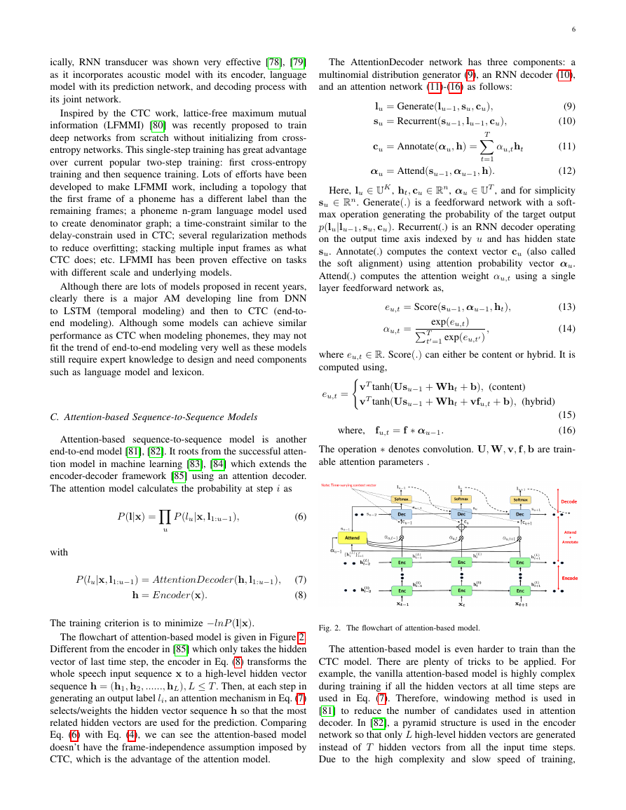
The flowchart of attention-based model is given in Figure 2.
Different from the encoder in [85] which only takes the hidden
vector of last time step, the encoder in Eq. (8) transforms the
whole speech input sequence x to a high-level hidden vector
sequence h = (h1, h2, ......, hL), L ≤ T . Then, at each step in
generating an output label li, an attention mechanism in Eq. (7)
selects/weights the hidden vector sequence h so that the most
related hidden vectors are used for the prediction. Comparing
Eq. (6) with Eq. (4), we can see the attention-based model
doesn’t have the frame-independence assumption imposed by
CTC, which is the advantage of the attention model.
Fig. 2. The flowchart of attention-based model.
The attention-based model is even harder to train than the
CTC model. There are plenty of tricks to be applied. For
example, the vanilla attention-based model is highly complex
during training if all the hidden vectors at all time steps are
used in Eq. (7). Therefore, windowing method is used in
[81] to reduce the number of candidates used in attention
decoder. In [82], a pyramid structure is used in the encoder
network so that only L high-level hidden vectors are generated
instead of T hidden vectors from all the input time steps.
Due to the high complexity and slow speed of training,
�
the majority of attention-based works were majorly done at
Google [82], compared to the CTC works reported from many
sites. However, recently Google significantly advanced the
research of attention-based model by
• modeling with word piece units [86] which are more
stable and helpful to LM modeling;
• including scheduled sampling [87] which feeds the pre-
vious predicted label instead of the ground truth during
training so that training and testing are consistent;
• having multi-head attention [88] so that each head can
generate a different attention distribution and play a
different role;
• applying label smoothing [89] to prevent the model from
making over-confident predictions;
• integrating external LM which was trained with more text
• using minimum word error rate sequence discriminative
data [90];
training [91].
With all these improvements, the final attention-based end-to-
end system clearly outperformed the traditional hybrid system
[92]. Different from CTC, a challenge to attention-based model
is the attention was performed on top of the whole input
utterance which means it cannot be performed in a streaming
fashion even if the encoder can be done in a streaming mode.
The frame-independence assumption in CTC is the most
criticized assumption as speech frames are correlated. On
the other hand, the attention-based model has its drawback
of not having monotonic left-to-right alignment and slow
convergence. In [93], the attention training is combined with
CTC training in a multi-task learning way by using CTC
objective function as the auxiliary function. Such a training
strategy greatly improves the convergence of attention-based
model and mitigates the alignment issue. In [94], it was further
advanced with jointly decoding with the scores from both
attention-based model and CTC model.
IV. ACOUSTIC MODEL ROBUSTNESS
Current state of the art systems can achieve remarkable
recognition accuracy when the test and training sets match,
esp. when both under quiet close-talk condition. However,
the performance dramatically degrades under mismatched or
complicated environments such as higher noise condition,
including music or interfering talkers, or speech with strong
accents [95], [96]. The solutions to this problem include
adaptation, speech enhancement, and robust modeling.
A. Acoustic Model Adaptation
In this section, we use speaker adaptation as an example
scenario to describe acoustic model adaptation technologies.
The same technology should be easily applied to the adaptation
of new environments and tasks, etc. Typically the speaker in-
dependent (SI) models are trained from a large dataset with an
objective to work best for all speakers. Speaker adaptation can
significantly boost the performance of an individual speaker
[97], [98]. However, we typically have limited adaptation
data, and unsupervised adaptation is the main stream given
7
prohibitive transcription cost. Current research focus is unsu-
pervised adaption with limited amount of speaker-dependent
data, which can be addressed with better adaptation criterion
and model topology. Since the adapted models are speaker
dependent (SD), the size of the SD parameters is critical if we
want to scale to millions of speakers. This requires solutions
to minimizing the SD model footprint while maintaining the
adaptation benefits.
Given the limited amount of adaptation data, the SD model
should not be far away from the SI model. [99] adds Kullback-
Leibler divergence (KLD) regularization to the training crite-
rion to prevent the adapted model from straying too far away
from the SI model. This KLD adaptation criterion has been
proven very effective dealing with limited adaption data. Most
state-of-the-art SI models use senone (tied triphone states)
as the output units. When limited amount of adaptation data
is available, only very small amount of senones have been
observed. In such a case, the adaptation turns to overfit the
data distribution of these senones thus cannot generalize very
well. In [100], a multi-task learning (MTL) framework was
proposed by adding auxiliary monophone classification as the
second task in addition to the primary seone classification
task. As a result, the network adaptation is backed off to
improving monophone classification accuracy when senones
are not observed, hence increasing the generalization ability.
In contrast to adjusting the adaptation criterion, most of
works focus on how to use very small amount of parameters to
represent speaker characteristics. One solution is the singular
value decomposition (SVD) bottleneck adaptation [101] which
produces low-footprint SD models by making use of the
SVD-restructured topology [102]. The linear transformation is
applied to each of the bottleneck layer by adding a kXk SD
matrices. The advantage of this approach is that only a couple
of small matrices need to be updated for each speaker as k is
the low-rank value of the SVD reconstruction and usually is
very small. This dramatically reduces the deployment cost for
speaker personalization while producing more reliable estimate
of the adapted model [101]. Works have been done to further
reduce the size of the kXk SD matrices. For example, when
the adaptation data is very limited, the kXk matrix can be
reduced to a diagonal matrix, such as learning hidden unit
contribution (LHUC) [103], [104] and sigmoid adaptation
[105]. This is a tradeoff between the modeling capacity
and generalization. The LHUC and sigmoid adaptation have
much smaller number of adaptation parameters compared to
the SVD adaption, but they may not get similar accuracy
improvement when the amount of adaptation data is increased.
The observation that kXk SD matrices usually are diagonally
dominant matrices inspired the proposal of low-rank plus
diagonal (LRPD) decomposition which decomposes the kXk
SD matrices into a diagonal matrix plus the multiplication
of two low-rank matrices. By varying the low-rank values,
the LPRD matrix generalizes the full-rank and the diagonal
adaptation matrix, and hence can automatically utilize the
adaptation data well instead of making tradeoff between model
capacity and generalization.
The subspace methods are another type of methods that also
aim to find a low dimensional subspace of the transformations,
�
so that each transformation can be specified by a small number
of parameters. One popular method in this category is the use
of auxiliary features, such as i-vector [106], [107], speaker
code [108] , and noise estimate [109] which are concatenated
with the standard acoustic features. It can be shown that the
augmentation of auxiliary features is equivalent to confining
the adapted bias vectors into a speaker subspace [110]. Fur-
thermore, networks can be used to transform speaker features
such as i-vectors into a bias to offset the speech feature into
a speaker-normalized space [111]. In addition to augmenting
features in the input space, the acoustic-factor features can
also be appended in any layer of deep networks [112].
Other subspace methods include cluster adaptive training
(CAT) [113], [114] and factorized hidden layer (FHL) [115],
[116], where the transformations are confined into the speaker
subspace. Similar to the eigenvoice [117] or cluster adaptive
training [118] in the Gaussian mixture model era, CAT [113],
[114] in DNN training constructs multiple DNNs to form the
bases of a canonical parametric space. During adaptation, an
interpolation vector which is associated to a target speaker
or environment is estimated online to combine the multiple
DNN bases into a single adapted DNN. Because only the
combination vector is estimated, the adaptation only needs
very small amount of data for fast adaptation. However, this
is again a tradeoff from the model capacity. In contrast with
online estimation of the combination vector, [119], [120]
directly uses the posterior vectors of the acoustic context
to enable fast unsupervised adaptation. The acoustic context
factor can be speaker, gender, or acoustic environments such
as noise and reverberation. The posterior calculation can be
either independent [119] or dependent [120] on the recognizer
network.
An issue in the CAT-style methods is that the bases are full-
rank matrices, which require very large amount of training
data. Therefore,
the number of bases in CAT is usually
constrained to few [113], [114]. A solution is to use FHL
[115], [116] which constrains the bases to be rank-1 matrices.
In such a way, the training data for each basis is significantly
reduced, enabling the use of larger number of bases. Also, FHL
initializes the combination vector from i-vector for speaker
adaptation, which helps to give the adaptation a very good
starting point. In [121], LRPD was extended into the subspace-
based approach to further reduce the speaker-specific footprint
in a very similar way to FHL.
B. Speech Enhancement and Separation
It is well known that the current ASR systems perform
poorly when the speech is corrupted with heavy noise or
interfering speech [122], [123]. Although human listeners also
suffer from poor audio signals, the performance degradation
is significantly smaller than that in ASR systems.
In recent years, many works have been done to enhance
speech under these conditions. Although majority of the works
are focused on single-channel speech enhancement and sepa-
ration, the same techniques can be easily extended to multi-
channel signals.
In the monaural speech enhancement and separation tasks,
it is assumed that a linearly mixed single-microphone signal
y[n] = S
8
s=1 xs[n] is known and the goal is to recover the
S streams of audio sources xs[n], s = 1,··· , S. If there
are only two audio sources, one for speech and one for
noise (or music, etc.) and the goal is to recover the speech
it’s often called speech enhancement. If there are
source,
multiple speech sources,
is often referred to as speech
separation. The enhancement and separation is usually carried
out
in which the task can
be cast as recovering the short-time Fourier transformation
(STFT) of the source signals Xs(t, f ) for each time frame t
and frequency bin f, given the STFT of the mixed speech
in the time-frequency domain,
it
Y (t, f ) =S
s=1 Xs(t, f ).
Obviously, given only the mixed spectrum Y (t, f ),
the
problem of recovering Xs(t, f ) is under-determined (or ill-
posed), as there are an infinite number of possible Xs(t, f )
combinations that lead to the same Y (t, f ). To overcome this
problem, the system has to learn a model based on some
training set S that contains parallel sets of mixtures Y (t, f )
and their constituent target sources Xs(t, f ), s = 1, ..., S [20],
[21], [124]–[129].
Over the decades, many attempts have been made to at-
tack this problem. Before the deep learning era, the most
popular techniques include computational auditory scene anal-
ysis (CASA) [130]–[132], non-negative matrix factorization
(NMF) [133]–[135], and model based approach [136]–[138],
such as factorial GMM-HMM [139]. Unfortunately these
techniques only led to very limited success.
Recently, researchers have developed many deep learning
techniques for speech enhancement and separation. The core
of these techniques is to cast the enhancement or separation
problem into a supervised learning problem. More specifically,
the deep learning models are optimized to predict the source
belonging to the target class, usually for each time-frequency
bin, given the pairs of (usually artificially) mixed speech and
source streams. Compared to the original setup of unsuper-
vised learning, this is a significant step forward and leads to
great progress in speech enhancement. This simple strategy,
however, is still not satisfactory, as it only works for separating
audios with very different characteristics, such as separating
speech from (often challenging) background noise (or music)
or speech of a specific speaker from other speakers [127].
It does not work well for speaker-independent multi-talker
speech separation.
The difficulty in speaker-independent multi-talker speech
separation comes from the label ambiguity or permutation
problem. Because audio sources are symmetric given the
mixture (i.e., x1 + x2 equals to x2 + x1 and both x1 and
x2 have the same characteristics), there is no pre-determined
way to assign the correct source target to the corresponding
output layer during supervised training. As a result, the model
cannot be well trained to separate speech.
Fortunately, several techniques have been proposed to ad-
dress the label ambiguity problem [20], [21], [123], [128],
[129], [140]. In Weng et al. [123] the instantaneous energy was
used to solve the label ambiguity problem and a two-speaker
joint-decoder with a speaker switching penalty was used to
separate and trace speakers. This work achieved the best
result on the dataset used in 2006 monaural speech separation
�


 2023年江西萍乡中考道德与法治真题及答案.doc
 2012年重庆南川中考生物真题及答案.doc
 2013年江西师范大学地理学综合及文艺理论基础考研真题.doc
 2020年四川甘孜小升初语文真题及答案I卷.doc
 2020年注册岩土工程师专业基础考试真题及答案.doc
 2023-2024学年福建省厦门市九年级上学期数学月考试题及答案.doc
 2021-2022学年辽宁省沈阳市大东区九年级上学期语文期末试题及答案.doc
 2022-2023学年北京东城区初三第一学期物理期末试卷及答案.doc
 2018上半年江西教师资格初中地理学科知识与教学能力真题及答案.doc
 2012年河北国家公务员申论考试真题及答案-省级.doc
 2020-2021学年江苏省扬州市江都区邵樊片九年级上学期数学第一次质量检测试题及答案.doc
 2022下半年黑龙江教师资格证中学综合素质真题及答案.doc