Probability
p
1.1 BASIC CONCEPTS
1.2 PROPERTIES OF PROBABILITY
1.3 METHODS OF ENUMERATION
1.4 CONDITIONAL PROBABILITY
1.5
1.6 BAYES'S THEOREM
INDEPENDENT EVENTS
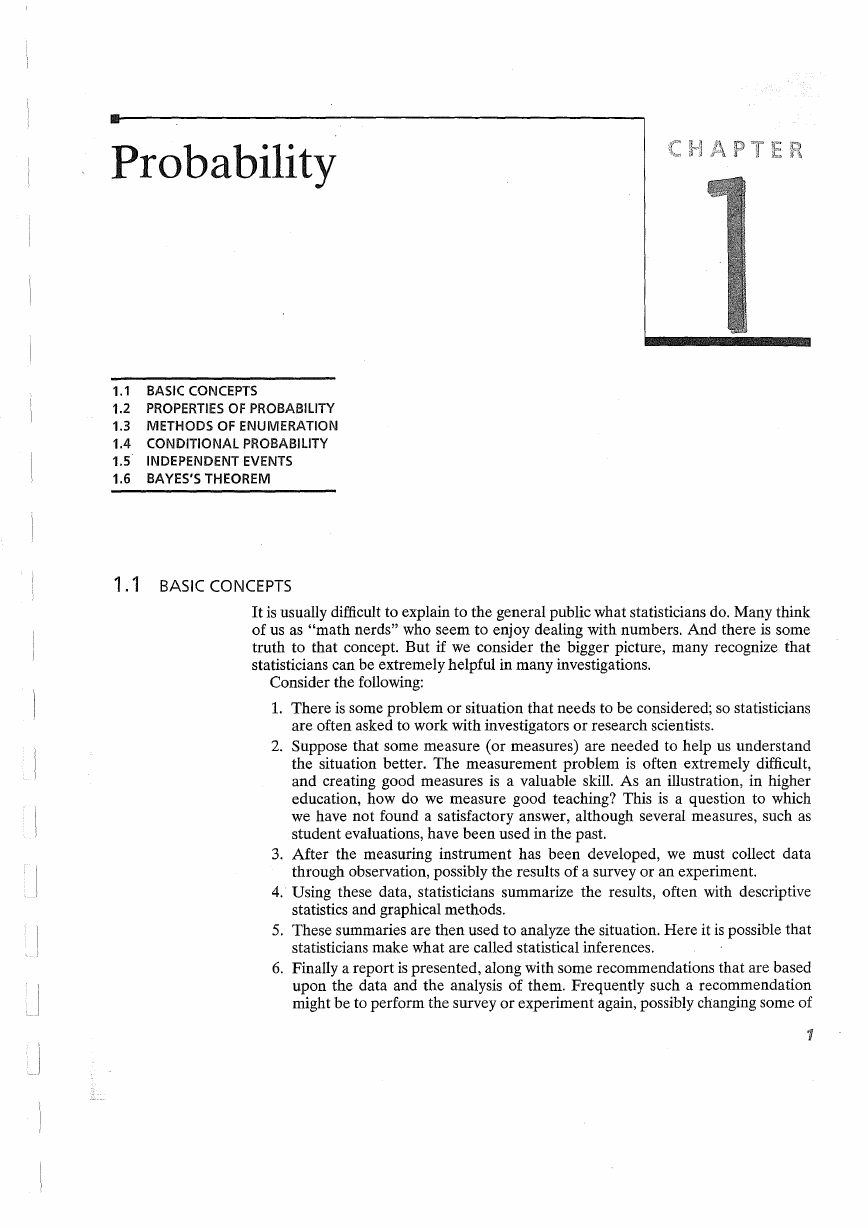
1. 1 BASIC CONCEPTS
It is usually difficult to explain to the general public what statisticians do. Many think
of us as "math nerds" who seem to enjoy dealing with numbers. And there is some
truth to that concept. But if we consider the bigger picture, many recognize that
statisticians can be extremely helpful in many investigations.
Consider the following:
1. There is some problem or situation that needs to be considered; so statisticians
are often asked to work with investigators or research scientists.
2. Suppose that some measure (or measures) are needed to help us understand
the situation better. The measurement problem is often extremely difficult,
and creating good measures is a valuable skill. As an illustration, in higher
education, how do we measure good teaching? This is a question to which
we have not found a satisfactory answer, although several measures, such as
student evaluations, have been used in the past.
3. After the measuring instrument has been developed, we must collect data
through observation, possibly the results of a surveyor an experiment.
4. Using these data, statisticians summarize the results, often with descriptive
statistics and graphical methods.
5. These summaries are then used to analyze the situation. Here it is possible that
statisticians make what are called statistical inferences.
6. Finally a report is presented, along with some recommendations that are based
upon the data and the analysis of them. Frequently such a recommendation
might be to perform the surveyor experiment again, possibly changing some of
1
�
I"'rooatllllty
the questions or factors involved. This is how statistics is used in what is referred
to as the scientific method, because often the analysis of the data suggests other
experiments. Accordingly, the scientist must consider different possibilities in
his or her search for an answer and thus performs similar experiments over and
over again.
The discipline of statistics deals with the collection and analysis of data. When
measurements are taken, even seemingly under the same conditions, the results
usually vary. Despite this variability, a statistician tries to find a patteI:n; yet due to
the "noise," not all of the data fit into the pattern. In the face of the variability, the
statistician must still determine the best way to describe the pattern. Accordingly,
statisticians know that mistakes will be made in data analysis, and they try to minimize
those errors as much as possible and then give bounds on the possible errors.
By considering these bounds, decision makers can decide how much confidence
they want to place in the data and in their analysis of them. If the bounds are
wide, perhaps more data should be collected. If, however, the bounds are narrow,
the person involved in the study might want to make a decision and proceed
accordingly.
Variability is a fact of life, and proper statistical methods can help us understand
data collected under inherent variability. Because of this variability, many decisions
have to be made that involve uncertainties. In medical research, interest may center
on the effectiveness of a new vaccine for mumps; an agronomist must decide whether
an increase in yield can be attributed to a new strain of wheat; a meteorologist
is interested in predicting the probability of rain; the state legislature must decide
whether decreasing speed limits will result in fewer accidents; the admissions officer
of a college must predict the college performance of an incoming freshman; a biologist
is interested in estimating the clutch size for a particular type of bird; an economist
desires to estimate the unemployment rate; an environmentalist tests whether new
controls have resulted in a reduction in pollution.
In reviewing the preceding (relatively short) list of possible areas of applications
of statistics, the reader should recognize that good statistics is closely associated with
careful thinking in many investigations. As an illustration, students should appreciate
how statistics is used in the endless cycle of the scientific method. We observe nature
and ask questions, we run experiments and collect data that shed light on these
questions, we analyze the data and compare the results of the analysis with what we
previously thought, we raise new questions, and on and on. Or if you like, statistics is
clearly part of the important "plan-do-study-act" cycle: Questions are raised and
investigations planned and carried out. The resulting data are studied and analyzed
and then acted upon, often raising new questions.
There are many aspects of statistics. Some people get interested in the subject by
collecting data and trying to make sense out of their observations. In some cases
the answers are obvious and little training in statistical methods is necessary. But
if a person goes very far in many investigations, he or she soon realizes that there
is a need for some theory to help describe the error structure associated with the
various estimates of the patterns. That is, at some point, appropriate probability
and mathematical models are required to make sense out of complicated data sets.
Statistics and the probabilistic foundation on which statistical methods are based can
provide the models to help people do this. So in this book, we are more concerned
with the mathematical, rather than the applied, aspects of statistics .. Still, we give
enough real examples so that the reader can get a good sense of a number of important
applications of statistical methods.
�
Section 1.1
Basic Concepts 3
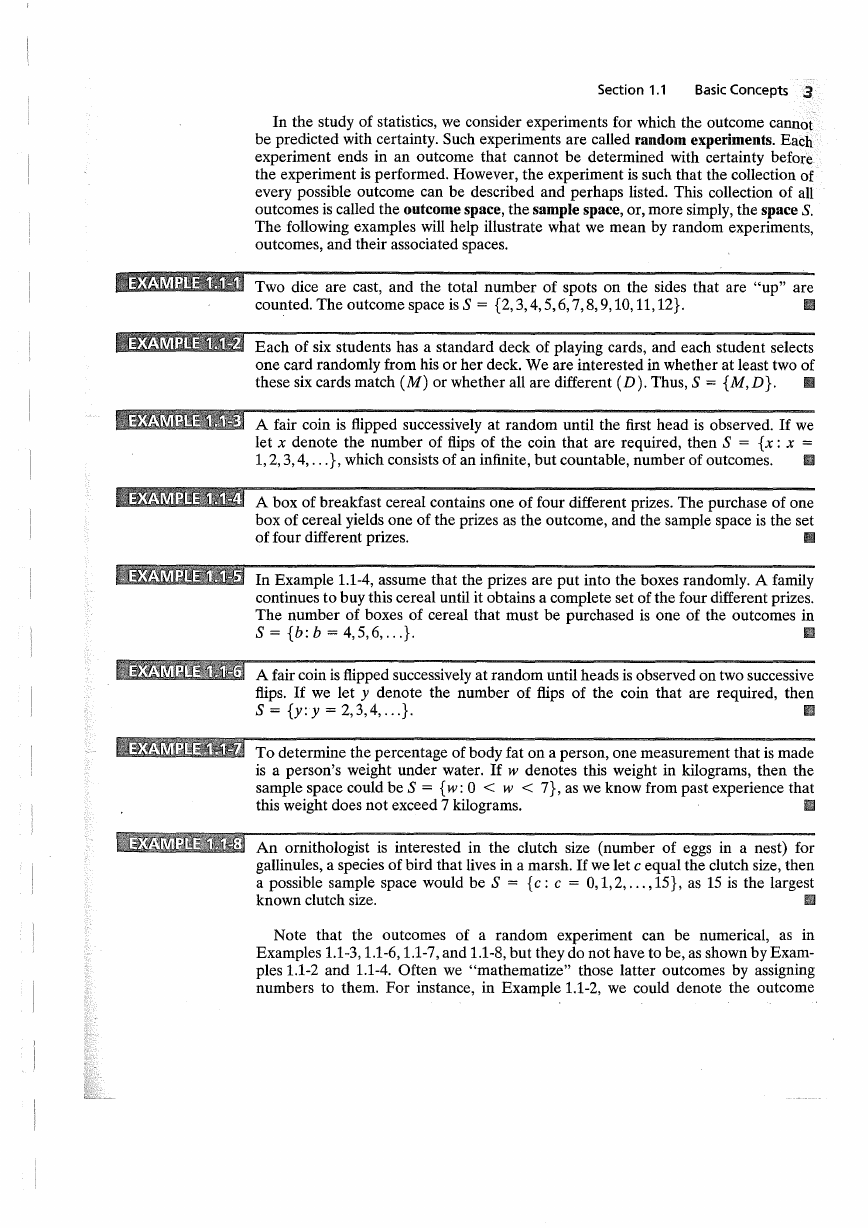
In the study of statistics, we consider experiments for which the outcome cannot
be predicted with certainty. Such experiments are called random experiments. Each
experiment ends in an outcome that cannot be determined with certainty before
the experiment is performed. However, the experiment is such that the collection of
every possible outcome can be described and perhaps listed. This collection of all
outcomes is called the outcome space, the sample space, or, more simply, the space S.
The following examples will help illustrate what we mean by random experiments,
outcomes, and their associated spaces .
• MMiUMilli Two dice are cast, and the total number of spots on the sides that are "up" are
11
counted. The outcome space is S = {2,3,4,5,6, 7,8, 9, 10, 11, 12}.
,#&liMU_il,) Each of six students has a standard deck of playing cards, and each student selects
one card randomly from his or her deck. We are interested in whether at least two of
these six cards match (M) or whether all are different (D). Thus, S = {M, D}.
11
.th'Mlijijlll1 A fair coin is flipped successively at random until the first head is observed. If we
let x denote the number of flips of the coin that are required, then S = {x: x =
1,2,3,4, ... }, which consists of an infinite, but countable, number of outcomes.
11
IW,;1MUMlliij A box of breakfast cereal contains one of four different prizes. The purchase of one
box of cereal yields one of the prizes as the outcome, and the sample space is the set
of four different prizes.
11
.t'liM~'11'1 In Example 1.1-4, assume that the prizes are put into the boxes randomly. A family
continues to buy this cereal until it obtains a complete set of the four different prizes.
The number of boxes of cereal that must be purchased is one of the outcomes in
S = {b: b = 4,5,6, ... }.
11
1#&i.i(tlYdiid A fair coin is flipped successively at random until heads is observed on two successive
flips. If we let y denote the number of flips of the coin that are required, then
S = {y: y = 2,3,4, ... }.
11
l#drllliim To determine the percentage of body fat on a person, one measurement that is made
sample space could be S = {w: ° < w < 7}, as we know from past experience that
is a person's weight under water. If w denotes this weight in kilograms, then the
this weight does not exceed 7 kilograms.
11
1#!it#3MiJr.illtl An ornithologist is interested in the clutch size (number of eggs in a nest) for
gallinules, a species of bird that lives in a marsh. If we let c equal the clutch size, then
a possible sample space would be S = {c: c = 0, 1,2, ... , 15}, as 15 is the largest
known clutch size.
11
Note that the outcomes of a random experiment can be numerical, as in
Examples 1.1-3, 1.1-6, 1.1-7, and 1.1-8, but they do not have to be, as shown by Exam
ples 1.1-2 and 1.1-4. Often we "mathematize" those latter outcomes by assigning
numbers to them. For instance, in Example 1.1-2, we could denote the outcome
�
4 Chapter 1
Probability
{D} by the number zero and the outcome {M} by the number one. In general,
measurements on outcomes associated with random experiments are called random
variables, and these are usually denoted by some capital letter toward the end of the
alphabet, such as X, Y, or Z.
Note the numbers of outcomes in the sample spaces in these examples. In Exam
ples 1.1-1,1.1-4, and 1.1-8, the number of outcomes is finite. In Examples 1.1-3 and
1.1-6, the number of possible outcomes is infinite but countable. That is, there are
as many outcomes as there are counting numbers (positive integers). The space for
Example 1.1-7 is different from that of the other examples in that the set of possible
outcomes is an interval of numbers. Theoretically the weight could be anyone of
an infinite number of possible weights; here the number of possible outcomes is not
countable. However, from a practical point of view, reported weights are selected
from a finite number of possibilities because we can read and record the answer
only to an accuracy determined by our scale. Many times, however, it is better to
conceptualize the space as an interval of outcomes, and Example 1.1-7 is an example
of a space of the continuous type.
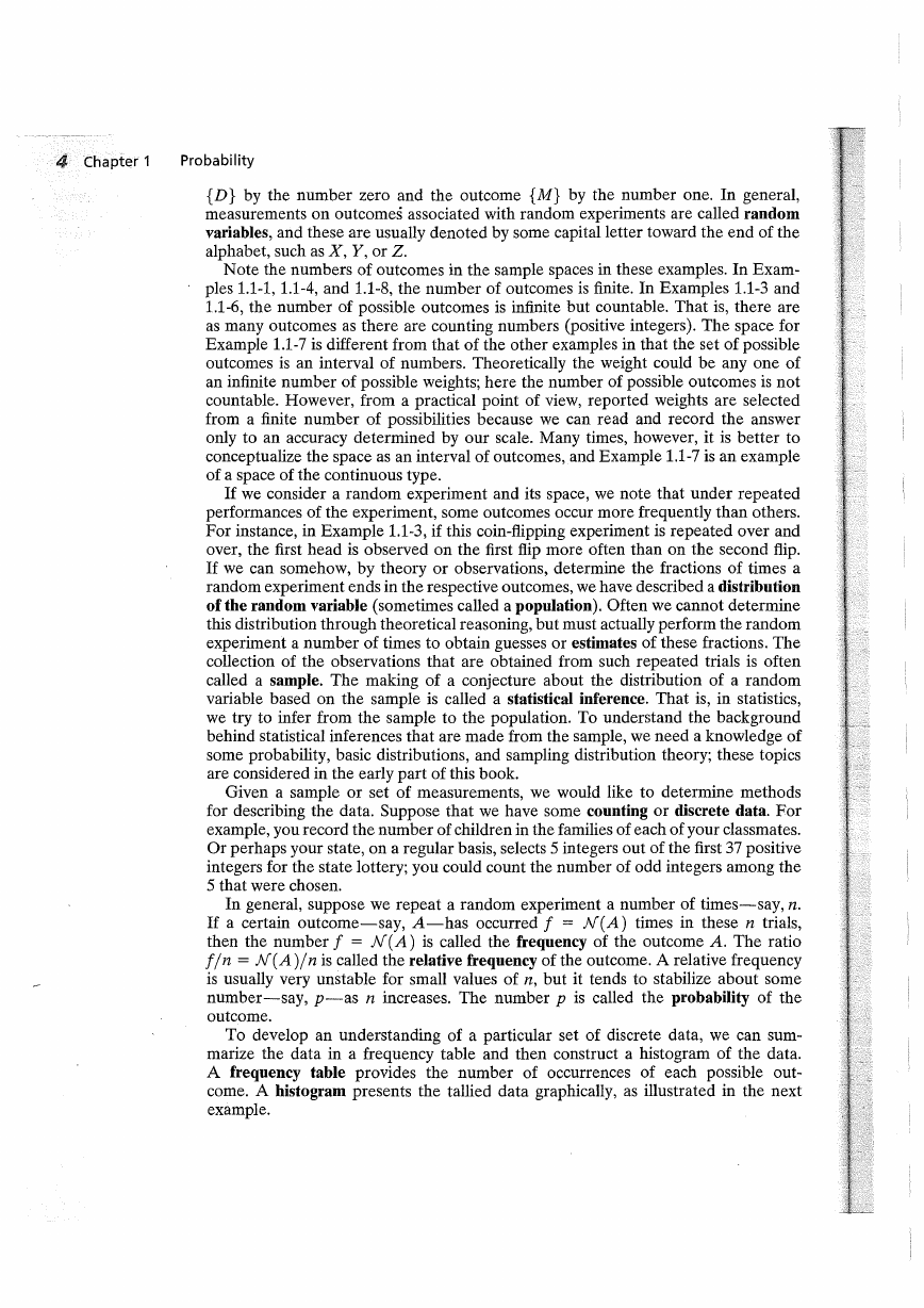
If we consider a random experiment and its space, we note that under repeated
performances of the experiment, some outcomes occur more frequently than others.
For instance, in Example 1.1-3, if this coin-flipping experiment is repeated over and
over, the first head is observed on the first flip more often than on the second flip.
If we can somehow, by theory or observations, determine the fractions of times a
random experiment ends in the respective outcomes, we have described a distribntion
of the random variable (sometimes called a popnlation). Often we cannot determine
this distribution through theoretical reasoning, but must actually perform the random
experiment a number of times to obtain guesses or estimates of these fractions. The
collection of the observations that are obtained from such repeated trials is often
called a sample. The making of a conjecture about the distribution of a random
variable based on the sample is called a statistical inference. That is, in statistics,
we try to infer from the sample to the population. To understand the background
behind statistical inferences that are made from the sample, we need a knowledge of
some probability, basic distributions, and sampling distribution theory; these topics
are considered in the early part of this book.
Given a sample or set of measurements, we would like to determine methods
for describing the data. Suppose that we have some counting or discrete data. For
example, you record the number of children in the families of each of your classmates.
Or perhaps your state, on a regular basis, selects 5 integers out of the first 37 positive
integers for the state lottery; you could count the number of odd integers among the
5 that were chosen.
In general, suppose we repeat a random experiment a number of times-say, n.
If a certain outcome-say, A-has occurred f = N(A) times in these n trials,
then the number f = N(A) is called the frequency of the outcome A. The ratio
f / n = N (A) / n is called the relative frequency of the outcome. A relative frequency
is usually very unstable for small values of n, but it tends to stabilize about some
number-say, p-as n increases. The number p is called the probability of the
outcome.
To develop an understanding of a particular set of discrete data, we can sum
marize the data in a frequency table and then construct a histogram of the data.
A frequency table provides the number of occurrences of each possible out
come. A histogram presents the tallied data graphically, as illustrated in the next
example.
�
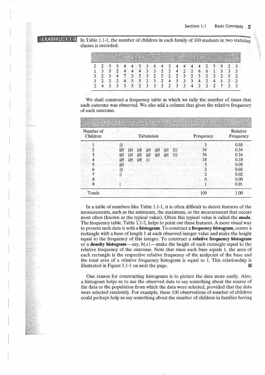
IEUMigMii14j In Table 1.1-1, the number of children in each family of 100 students in two statistics
classes is recorded.
Section 1.1
Basic Concepts 5
2 2 5 3 4 4 3 3
1 3 5 2 4 4 4 3 3 2 2 4 2 2
,
3 2
3 4
3 2
2 2 4 3 3
2 4 3 3 3 5 2
6 4 3 4 4 4 4 2 5 9 2 3
6 1 3 3 3
3 3 2 2 2 2 3 2 3 2 3 2 5 2
2 3 2
2 2
3 3 2 2 3 3 4 2 2 2 7 2 3
7 3
6
4 3 3 3 4 2 4 1
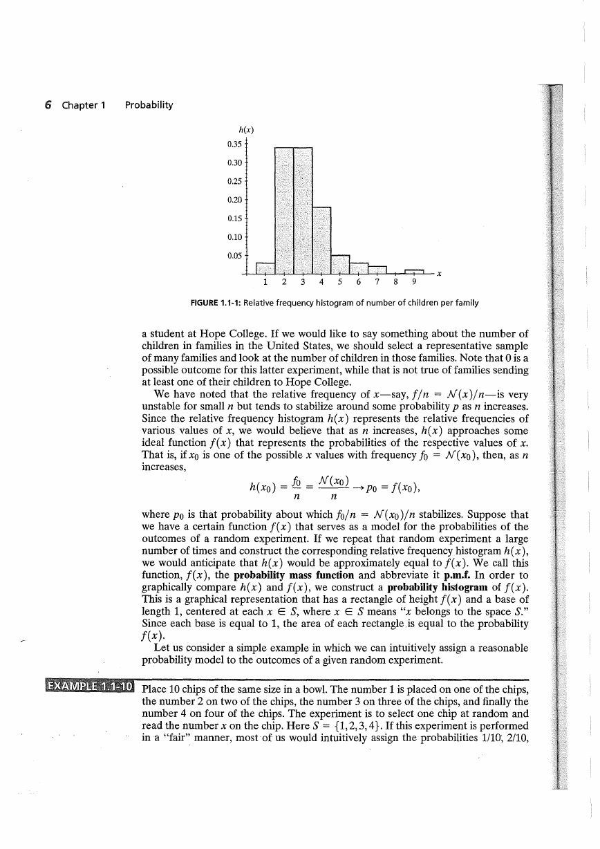
We shall construct a frequency table in which we tally the number of times that
each outcome was observed. We also add a column that gives the relative frequency
of each outcome.
Number of
Children
Tabulation
Frequency
Relative
Frequency
III
wt wt wt wt wt wt
wt wt wt AA wt wt
wt wt wt
wt
III
11
III
I11I
11I1
1
2
3
4
5
6
7
8
9
Totals
3
34
34
18
5
3
2
0
1
100
0.03
0.34
0.34
0.18
0.05
0.03
0.02
0.00
0.01
1.00
In a table of numbers like Table 1.1-1, it is often difficult to detect features of the
measurements, such as the minimum, the maximum, or the measurement that occurs
most often (known as the typical value). Often this typical value is called the mode.
The frequency table, Table 1.1-2, helps to point out these features. A more visual way
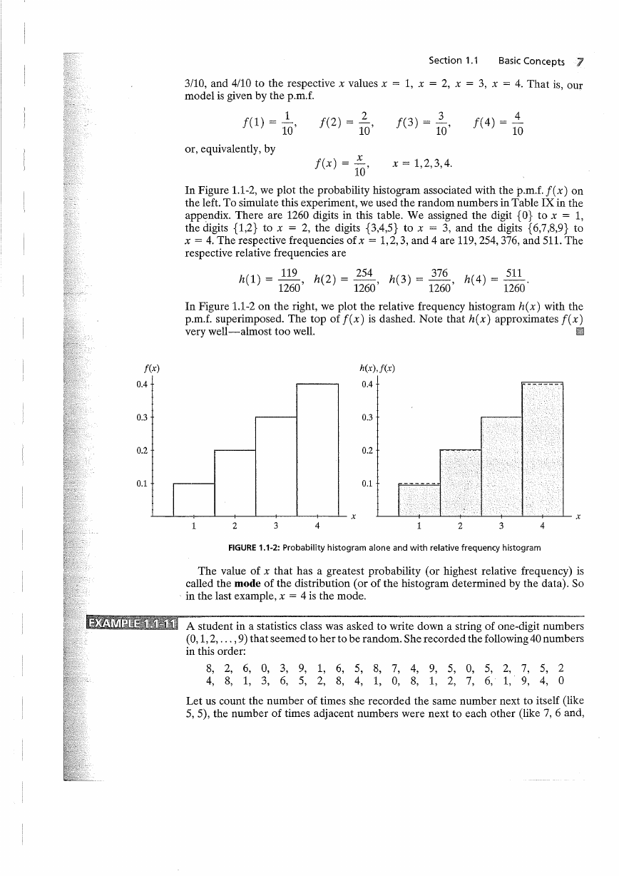
to present such data is with a histogram. To construct a frequency histogram, center a
rectangle with a base of length 1 at each observed integer value and make the height
equal to the frequency of this integer. To construct a relative frequency histogram
or a density histogram-say, hex )-make the height of each rectangle equal to the
relative frequency of the outcome. Note that since each base equals 1, the area of
each rectangle is the respective relative frequency of the midpoint of the base and
the total area of a relative frequency histogram is equal to 1. This relationship is
III
illustrated in Figure 1.1-1 on next the page.
One reason for constructing histograms is to picture the data more easily. Also,
a histogram helps us to use the observed data to say something about the source of
the data or the popUlation from which the data were selected, provided that the data
were selected randomly. For example, these 100 observations of number of children
could perhaps help us say something about the number of children in families having
�
6 Chapter 1
Probability
h(x)
0.35
0.30
0.25
0.20
0.15
0.10
0.05
1
2
3
4
5
6
7
8
9
x
FIGURE 1.1-1: Relative frequency histogram of number of children per family
a student at Hope College. If we would like to say something about the number of
children in families in the United States, we should select a representative sample
of many families and look at the number of children in those families. Note that 0 is a
possible outcome for this latter experiment, while that is not true of families sending
at least one of their children to Hope College.
We have noted that the relative frequency of x-say, fin = N(x)ln-is very
unstable for small n but tends to stabilize around some probability P as n increases.
Since the relative frequency histogram h(x) represents the relative frequencies of
various values of x, we would believe that as n increases, h (x) approaches some
ideal function f( x) that represents the probabilities of the respective values of x.
That is, if Xo is one of the possible x values with frequency fo = N (xo ), then, as n
increases,
h(xo) = fo = N(xo) ~ Po = f(xo),
n
n
where Po is that probability about which foln = N(xo)ln stabilizes. Suppose that
we have a certain function f( x) that serves as a model for the probabilities of the
outcomes of a random experiment. If we repeat that random experiment a large
number of times and construct the corresponding relative frequency histogram h (x),
we would anticipate that h(x) would be approximately equal to f(x). We call this
function, f(x), the probability mass function and abbreviate it p.m.f. In order to
graphically compare h(x) and f(x), we construct a probability histogram of f(x).
This is a graphical representation that has a rectangle of height f(x) and a base of
length 1, centered at each x E S, where x E S means "x belongs to the space S."
Since each base is equal to 1, the area of each rectangle.is equal to the probability
f(x).
Let us consider a simple example in which we can intuitively assign a reasonable
probability model to the outcomes of a given random experiment.
iDliMnllli.j Place 10 chips of the same size in a bowl. The number 1 is placed on one of the chips,
the number 2 on two of the chips, the number 3 on three of the chips, and finally the
number 4 on four of the chips. The experiment is to select one chip at random and
read the number x on the chip. Here S = {1, 2, 3, 4}. If this experiment is performed
ina "fair" manner, most of us would intuitively assign the probabilities lIW, 2/10,
�
Section 1.1
Basic Concepts 7
3110, and 4110 to the respective x values x = 1, x = 2, x = 3, x = 4. That is, our
model is given by the p.m.f.
1
f(l) = 10'
2
f(2) = 10'
3
f(3) = 10'
f(4) = -
4
10
or, equivalently, by
x
f(x) = 10'
x = 1,2,3,4.
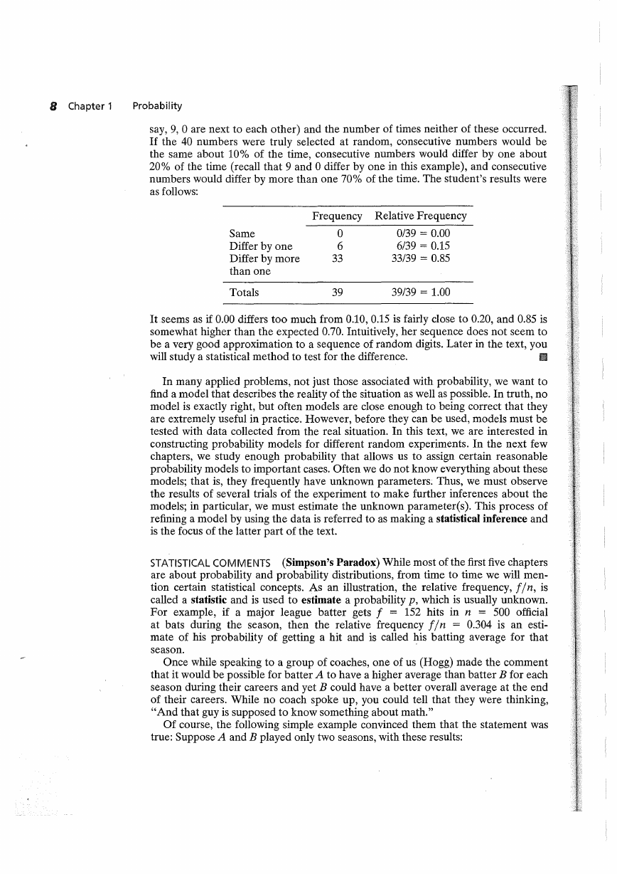
In Figure 1.1-2, we plot the probability histogram associated with the p.m.f. f(x) on
the left. To simulate this experiment, we used the random numbers in Table IX in the
appendix. There are 1260 digits in this table. We assigned the digit {O} to x = 1,
the digits {1,2} to x = 2, the digits {3,4,5} to x = 3, and the digits {6,7,8,9} to
x = 4. The respective frequencies of x = 1,2,3, and 4 are 119,254,376, and 511. The
respective relative frequencies are
h(l) = 119
1260'
h(2) = 254
1260'
h(3) = 376
1260'
h( 4) = 511.
1260
In Figure 1.1-2 on the right, we plot the relative frequency histogram h(x) with the
p.m.f. superimposed. The top of f( x) is dashed. Note that h( x) approximates f( x)
very well-almost too well.
III
f(x)
0.4
0.3
0.2
0.1
h(x),f(x)
0.4
0.3
0.2
0.1
x
1
2
3
4
1
2
3
4
x
FIGURE 1.1-2: Probability histogram alone and with relative frequency histogram
The value of x that has a greatest probability (or highest relative frequency) is
called the mode of the distribution (or of the histogram determined by the data). So
. in the last example, x = 4 is the mode.
A student in a statistics class was asked to write down a string of one-digit numbers
(0,1,2, ... ,9) that seemed to her to be random. She recorded the following 40 numbers
in this order:
8, 2, 6, 0, 3, 9, 1, 6, 5, 8, 7, 4, 9, 5, 0, 5, 2, 7, 5, 2
4, 8, 1, 3, 6, 5, 2, 8, 4, 1, 0, 8, 1, 2, 7, 6, 1,· 9, 4, °
Let us count the number of times she recorded the same number next to itself (like
5,5), the number of times adjacent numbers were next to each other (like 7, 6 and,
�
8 Chapter 1
Probability
say, 9, 0 are next to each other) and the number of times neither of these occurred.
If the 40 numbers were truly selected at random, consecutive numbers would be
the same about 10% of the time, consecutive numbers would differ by one about
20% of the time (recall that 9 and 0 differ by one in this example), and consecutive
numbers would differ by more than one 70% of the time. The student's results were
as follows:
Frequency
Relative Frequency
Same
Differ by one
Differ by more
than one
Totals
o
6
33
39
0/39 = 0.00
6/39 = 0.15
33/39 = 0.85
39/39 = 1.00
It seems as if 0.00 differs too much from 0.10, 0.15 is fairly close to 0.20, and 0.85 is
somewhat higher than the expected 0.70. Intuitively, her sequence does not seem to
be a very good approximation to a sequence of random digits. Later in the text, you
11
will study a statistical method to test for the difference.
In many applied problems, not just those associated with probability, we want to
find a model that describes the reality of the situation as well as possible. In truth, no
model is exactly right, but often models are close enough to being correct that they
are extremely useful in practice. However, before they can be used, models must be
tested with data collected from the real situation. In this text, we are interested in
constructing probability models for different random experiments. In the next few
chapters, we study enough probability that allows us to assign certain reasonable
probability models to important cases. Often we do not know everything about these
models; that is, they frequently have unknown parameters; Thus, we must observe
the results of several trials of the experiment to make further inferences about the
models; in particular, we must estimate the unknown parameter(s). This process of
refining a model by using the data is referred to as making a statistical inference and
is the focus of the latter part of the text.
(Simpson's Paradox) While most of the first five chapters
STATISTICAL COMMENTS
are about probability and probability distributions, from time to time we will men
tion certain statistical concepts. As an illustration, the relative frequency, t/ n, is
called a statistic and is used to estimate a probability p, which is usually unknown.
For example, if a major league batter gets f = 152 hits in n = 500 official
at bats during the season, then the relative frequency fin = 0.304 is an esti
mate of his probability of getting a hit and is called his batting average for that
season.
Once while speaking to a group of coaches, one of us (Hogg) made the comment
that it would be possible for batter A to have a higher average than batter B for each
season during their careers and yet B could have a better overall average at the end
of their careers. While no coach spoke up, you could tell that they were thinking,
"And that guy is supposed to know something about math."
Of course, the following simple example convinced them that the statement was
true: Suppose A and B played only two seasons, with these results:
�


 2023年江西萍乡中考道德与法治真题及答案.doc
 2012年重庆南川中考生物真题及答案.doc
 2013年江西师范大学地理学综合及文艺理论基础考研真题.doc
 2020年四川甘孜小升初语文真题及答案I卷.doc
 2020年注册岩土工程师专业基础考试真题及答案.doc
 2023-2024学年福建省厦门市九年级上学期数学月考试题及答案.doc
 2021-2022学年辽宁省沈阳市大东区九年级上学期语文期末试题及答案.doc
 2022-2023学年北京东城区初三第一学期物理期末试卷及答案.doc
 2018上半年江西教师资格初中地理学科知识与教学能力真题及答案.doc
 2012年河北国家公务员申论考试真题及答案-省级.doc
 2020-2021学年江苏省扬州市江都区邵樊片九年级上学期数学第一次质量检测试题及答案.doc
 2022下半年黑龙江教师资格证中学综合素质真题及答案.doc