The Gravity of the Opioid Crisis
The United States is in the midst of a national crisis due to the extreme abuse
of opioids all across the country. More than ever before, users of all ages and demo-
graphics are becoming addicted. To explore future impacts of this drug epidemic, we
model and characterize the spread of substance abuse.
We use NFLIS drug report data 2010-2017 to develop a multivariate analysis of
the spread of drug use in and between counties of Kentucky, Ohio, Pennsylvania,
Virginia, and West Virginia. We base the development of the drug spread model on
three main factors:
i. Drug-use influence
ii. Current trend in drug reports
iii. Pertinent socio-economic factors
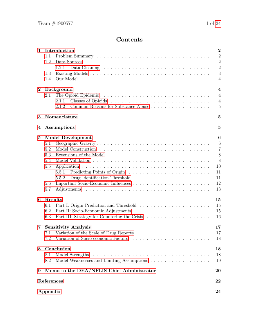
We identify the current trend of drug reports by implementing a quadratic-weighted
linear regression on existing county drug report data across time. To characterize the
nature of drug-use influence on a county, we define a county’s drug influence factor
as the density of drug reports per area. We find the origins of specific opioids and de-
termine the drug identification thresholds based on the influence factor. Six counties
crossed our determined threshold for our simulation from 2018 to 2025, indicating
that the epidemic is increasing in intensity.
Using the principles of geographic gravity, we establish an inverse relationship
between influence on other counties and distance as a weighted factor of their existing
trend. We validate our model as a better predictor of the following year’s drug reports
than the data from the previous year.
We then find associations between drug reports and U.S. Census socio-economic
factors over time. With the highest correlated socio-economic data, we calculate
a multivariate linear regression of the drug reports based on time. This adjusted
model shows a 12.2% decrease in residuals of our predicted data against the real
data, compared to the baseline.
We use strategies from other parts of the United States to make improvements
in accommodating drug users. Using factors such as drug education and recovery
centers, we estimate a reduction in overall drug consumption.
�
Team #1900577
1 of 24
Contents
1 Introduction
1.1 Problem Summary . . . . . . . . . . . . . . . . . . . . . . . . . . . . . . . .
. . . . . . . . . . . . . . . . . . . . . . . . . . . . . . . . . . .
1.2 Data Sources
1.2.1 Data Cleaning . . . . . . . . . . . . . . . . . . . . . . . . . . . . . .
1.3 Existing Models . . . . . . . . . . . . . . . . . . . . . . . . . . . . . . . . . .
. . . . . . . . . . . . . . . . . . . . . . . . . . . . . . . . . . . .
1.4 Our Model
2 Background
2.1 The Opioid Epidemic . . . . . . . . . . . . . . . . . . . . . . . . . . . . . . .
2.1.1 Classes of Opioids
. . . . . . . . . . . . . . . . . . . . . . . . . . . .
2.1.2 Common Reasons for Substance Abuse . . . . . . . . . . . . . . . . .
3 Nomenclature
4 Assumptions
5 Model Development
5.1 Geographic Gravity . . . . . . . . . . . . . . . . . . . . . . . . . . . . . . . .
5.2 Model Construction . . . . . . . . . . . . . . . . . . . . . . . . . . . . . . .
5.3 Extensions of the Model
. . . . . . . . . . . . . . . . . . . . . . . . . . . . .
5.4 Model Validation . . . . . . . . . . . . . . . . . . . . . . . . . . . . . . . . .
5.5 Application . . . . . . . . . . . . . . . . . . . . . . . . . . . . . . . . . . . .
5.5.1 Predicting Points of Origin . . . . . . . . . . . . . . . . . . . . . . .
5.5.2 Drug Identification Threshold . . . . . . . . . . . . . . . . . . . . . .
Important Socio-Economic Influences . . . . . . . . . . . . . . . . . . . . . .
. . . . . . . . . . . . . . . . . . . . . . . . . . . . . . . . . . .
5.6
5.7 Adjustments
6 Results
6.1 Part I: Origin Prediction and Threshold . . . . . . . . . . . . . . . . . . . .
6.2 Part II: Socio-Economic Adjustments . . . . . . . . . . . . . . . . . . . . . .
6.3 Part III: Strategy for Countering the Crisis
. . . . . . . . . . . . . . . . . .
7 Sensitivity Analysis
7.1 Variation of the Scale of Drug Reports . . . . . . . . . . . . . . . . . . . . .
7.2 Variation of Socio-economic Factors
. . . . . . . . . . . . . . . . . . . . . .
8 Conclusion
8.1 Model Strengths
. . . . . . . . . . . . . . . . . . . . . . . . . . . . . . . . .
8.2 Model Weaknesses and Limiting Assumptions . . . . . . . . . . . . . . . . .
9 Memo to the DEA/NFLIS Chief Administrator
References
Appendix
2
2
2
2
3
4
4
4
4
5
5
5
6
6
7
8
8
10
11
11
12
13
15
15
15
16
17
17
18
18
18
19
20
22
24
�
Team #1900577
2 of 24
1
Introduction
Drug abuse is an issue that the world has been plagued with for centuries. The
first study of morphine addiction was done in 1875, identifying the key factors for
a user to become addicted to a substance [13]. In the past several decades in the
United States, the opioid epidemic has increased at an alarming rate. Currently, an
average of 130 citizens of the U.S die of an opioid overdose daily [4]. Understanding
the spread of this epidemic can be used to inform government policy to get control
of this crisis.
1.1 Problem Summary
For the U.S. government, it is a challenge to enforce anti-drug laws, especially amid
the national crisis that is happening. The Drug Enforcement Administration (DEA)
wishes to see if there are factors that contribute to the spread of opioid incidents
between 5 states in the eastern United States — Ohio (OH), Kentucky (KY), West
Virginia (WV), Virginia (VA), and Pennsylvania (PA).
We use data analysis to build a model that describes the spread of opioid cases
in these states, with the ability to identify any possible locations where a specific
drug might have originated. We then set a threshold which signifies an unsafe level
of drug use in the county, predicting where this will occur in the future. We then
add U.S. Census data to our model, implementing socio-economic factors into the
model. When then use this model to identify strategies for countering the opioid
epidemic, and test the effectiveness of these strategies.
1.2 Data Sources
Our model is informed by 8 years worth of drug identification counts, 2010 to 2017,
for narcotic analgesics and heroin from the National Forensic Laboratory Information
System (NFLIS). We also derived geographic data from the NFLIS dataset [9]. The
model is conditioned with 7 years worth of data from the U.S. Census Bureau, 2010
to 2016, that represents a common set of socio-economic factors.
1.2.1 Data Cleaning
The census data provided had missing and partially filled in data that would have
been challenging to effectively utilize. We did the following to sanitize the data-set:
- Remove factors that were not measured at all (represented by the symbol (x),
such as HC04 VC03)
�
Team #1900577
3 of 24
- Remove factors that were only measured in certain years, such as computers
and internet use (HC01 VC216), as trends across multiple years would be less
present and more susceptible to potential outliers.
- Remove factors that had incomplete data for all the counties, often represented
by the symbol “*****”. Incomplete data for a factor would inhibit the creation
of a proper model for drug spread, as there could be hidden trends that are not
apparent because of missing data.
1.3 Existing Models
Many comprehensive studies and models of drug spread and impact have been
executed in the past. Many of these models focus on the following ideas:
• Illicit drug users are broken into 3 groups:
light users, susceptible users, and
dealers. Each of these groups may enter any of the others through remission,
death, or influence [7].
• Set a threshold quantity to how many new drug abusers an average dealer or
• Predict future changes by modeling the previous waves of the opioid epidemic.
The first wave began in 1999 with prescription opioids, the second started in
2010 with a rise in heroin use, and the third commenced in 2013 with synthetic
opioids becoming more common, as can be seen in Figure 1.
light user will generate over their lifetime [12].
Figure 1: The three waves of the opioid epidemic [2]
�
Team #1900577
1.4 Our Model
4 of 24
For the purpose of determining an effective model to describe the spread of opioid
incidents, we characterized the nature of drug-use influence on each county, both
externally and internally. External influence on a county is determined by the density
of drug reports of nearby counties, inversely related by geographic distance. Internally,
a county’s influence comes from a weighted trend analysis of total drug reports
based on category.
With the addition of socio-economical factors, our model took a multi-variate
approach. We determined which factors had the greatest impact on the trends
in drug use, and applied a predictive fit to determine how changes in these factors
influence a county. This will allow us to predict how the spread of drug reports will
change in the future, creating the opportunity to mitigate the opioid epidemic before
it grows more out of control.
2 Background
2.1 The Opioid Epidemic
The opioid epidemic is a strange phenomenon of drug addiction where people
begin taking prescription opioids for pain management related to a medical issue [5].
By nature, opioids are a highly addictive form of drug, and a user can quickly become
dependent due the euphoric feeling they experience while taking them. Users quickly
build up a tolerance to this drug, and require more or different types for them to
continue to be effective [2]. This can cause issues, especially in medical treatment, as
a user’s body will no longer respond to certain forms of this drug, causing great pain.
2.1.1 Classes of Opioids
There are three main classes of opioids:
- Opiates (non-synthetic opioids): codeine, morphine, opium, heroin
- Semi-synthetic opioids: Hydrocodone, oxycodone, buprenorphine
- Synthetic opioids: Fentanyl, butorphanol, methadone, propoxyphene
This distinction in type of opioid different users will use each category, which can re-
sult in varying overall trends. Although heroin is considered an opiate, it is processed
from morphine and typically placed in its own category for analysis.
Strength of opioids are compared with an Oral Morphine Milligram Equivalent
(MME) Conversion Factor. For example, the synthetic opioid tramadol has a 0.1
MME conversion factor, meaning tramadol is 10 times stronger than the equivalent
�
Team #1900577
5 of 24
mass of morphine. The trend is that synthetic opioids are much stronger in their
effects than opiates and semi-synthetic opioids.
2.1.2 Common Reasons for Substance Abuse
There are several factors that researchers generally attribute to increasing the
likelihood of addiction [6]:
- Mental Health Problems
- Career, home, school, or friendship issues
- Proximity to other drug users
- Past traumatic events
3 Nomenclature
Symbol
Definition
Gd,i
Ii
Pi
RE
r
Imax
i
m
ri,j
Si
∆Drug
∆φ
∆λ
φ1
φ2
µI
Gravity of Influence for drug d and county i
Influence factor of a county i
External influence on county i
Radius of the Earth
Distance along the earth in kilometers
Largest influence factor in the data set
County identifier
Time derivative of linear best fit in drugs vs time
Distance between counties i and j (m)
Set containing every county identifier excluding i
Predicted change in drug reports
Difference of latitudes in radians
Difference of longitudes in radians
Radian measure of latitude 1
Radian measure of latitude 2
Median influence factor
Table 1: Variables and functions
4 Assumptions
• Illicit drug use is primarily influenced by human interaction. Like culture, drug
use will spread geographically, more strongly affecting nearby locations than
those far away [8].
�
Team #1900577
6 of 24
• The drug report data is representative of overall drug usage in a county or state.
• Smaller (rural) populations will be more susceptible to change based outside
influences than larger (urban) populations.
• New types of drugs generally appear in waves, which is uncertain to predict
based on the drug report data provided. For the purpose of this model, we
assume that no new drugs will be introduced to the population.
• Without external influence, an addicted population will continue their current
trend of drug use [10].
5 Model Development
In order to quantify and predict the rate of opioid spread between these 5 states,
it is necessary to justify the idea of influence. One of the largest factors that increase
the likelihood of drug addiction is proximity to to other drug uses. A county, in some
capacity, will be more strongly affected by the drug use of counties nearby than by
those that are farther away. To quantify the density of drug use in an area, we define
the influence factor for a county i:
Ii =
Number of Drug Reports in County i
Area of County i
(1)
Assuming that the count of drug reports in an area properly represents the actual
drug use in that area, we can use this factor as a standardized way to measure drug
use in a county. The hypothesis that the spread of the opioid epidemic is correlated
to drug reports density rather than strictly the magnitude of these values parallels
work previously done in epidemiology [15].
5.1 Geographic Gravity
The next step is to determine the impact of these influences on neighboring coun-
ties. We begin with the idea of gravity. In physics, the force of gravity on an object
is proportional to the product of the mass of each object divided by the distance
between the two objects squared:
Fg ∝ m1m2
r2
(2)
Much like how this quantity is dependent on the inverse square of the distance
between to objects, the drug influence of a county on another decreases with the dis-
tance from the county as well. Yanguang Chen’s work in spatial analysis in geography
�
Team #1900577
7 of 24
and social physics upholds this idea, stating that a gravitational model illustrates the
interaction between counties, while a exponential decay is more suggestive of local
rather than spatial interaction [8].
In order for our model to measure distance, we need to utilize external geograph-
ical data. We used the FIPS codes provided in the data to match each county with a
latitude coordinate, longitude coordinate, and county land area from the U.S. Census
Bureau [9]. Although these coordinates point to the center of each county (which
may not be completely representative for an unusually-shaped county’s location), it
provides us with a method to determine distances between counties. We now use
the Haversine formula to determine the distance between any two counties, which
accounts for Earth’s curvature to provide a more accurate value than Cartesian esti-
mation:
a = sin2∆φ
+ cos(φ1) cos(φ2) sin2∆λ
√
a),
r = 2RE arcsin(
2
2
Equipped with a measure of a county’s drug influence, along with the distance
between each county, we define the External Influence Potential on county i as:
Pi =
, Si = {j ∈ N | 1 ≤ j ≤ n; j = i}
Ij
r2
i,j
(3)
j�Si
5.2 Model Construction
Our opioid spread model focuses on two main ideas: a county’s influence (both
internal and external) along with the current trend of county drug reports with respect
to time. Although it would have been beneficial to have more extensive historical data,
we utilized the 8 years’ worth of NFLIS to determine the current drug report trend
in a county with reasonable accuracy.
To find this trend, we perform a weighted trend analysis for each county. We apply
a linear fit to the total county drug reports with respect to time using a quadratic
weight of (year − 2009)2 for each point up to the current year. This allows us to
take into account a county’s past drug report use, while also placing a much higher
significance on more recent trends in the data. The time-derivative of this linear fit
mi is calculated for every year and county for which there were at least two years’
worth of drug report data.
In order to combine influence factors with current trends in the data, we introduce
a normalization coefficient for the influence values. This coefficient serves to normal-
ize these influence values, along with providing a basis for how much the external
influence potential will affect the change in drug reports for that county. Based on
models of social physics, a county with a large influence will be much affected much
�




 2023年江西萍乡中考道德与法治真题及答案.doc
 2012年重庆南川中考生物真题及答案.doc
 2013年江西师范大学地理学综合及文艺理论基础考研真题.doc
 2020年四川甘孜小升初语文真题及答案I卷.doc
 2020年注册岩土工程师专业基础考试真题及答案.doc
 2023-2024学年福建省厦门市九年级上学期数学月考试题及答案.doc
 2021-2022学年辽宁省沈阳市大东区九年级上学期语文期末试题及答案.doc
 2022-2023学年北京东城区初三第一学期物理期末试卷及答案.doc
 2018上半年江西教师资格初中地理学科知识与教学能力真题及答案.doc
 2012年河北国家公务员申论考试真题及答案-省级.doc
 2020-2021学年江苏省扬州市江都区邵樊片九年级上学期数学第一次质量检测试题及答案.doc
 2022下半年黑龙江教师资格证中学综合素质真题及答案.doc