Open Journal of Applied Sciences, 2017, 7, 115-128
http://www.scirp.org/journal/ojapps
ISSN Online: 2165-3925
ISSN Print: 2165-3917
Driving Style Recognition Based on Driver
Behavior Questionnaire
Pengfei Li1*, Jianjun Shi1, Xiaoming Liu2
1Key Laboratory of Traffic Engineering, Beijing University of Technology, Beijing, China
2Ministry of Transport of the People’s Republic of China, Beijing, China
How to cite this paper: Li, P.F., Shi, J.J.
and Liu, X.M. (2017) Driving Style Recog-
nition Based on Driver Behavior Ques-
tionnaire. Open Journal of Applied Sci-
ences, 7, 115-128.
https://doi.org/10.4236/ojapps.2017.74010
Received: February 16, 2017
Accepted: April 21, 2017
Published: April 25, 2017
Copyright © 2017 by authors and
Scientific Research Publishing Inc.
This work is licensed under the Creative
Commons Attribution International
License (CC BY 4.0).
http://creativecommons.org/licenses/by/4.0/
Open Access
Abstract
The ability to classify driver behavior lays the foundation for more advanced
driver assistance systems. The present study aims to research driver pattern
and classification feature. Driver behavior self-reported investigation was
conducted with standardized driver behavior questionnaire (DBQ) by 225
nonprofessional drivers on the internet in Beijing. Questionnaire’s reliability
was verified by statistics analysis. Confirmatory factor analysis (CFA) was
used to analyze the underlying factor structure. Speed advantage, space occu-
pation, the contend right of way and the contend space advantage were ex-
tracted from the questionnaire results to quantify driver characteristics. Based
on fuzzy C-means (FCM) algorithm and taking the four factors as pattern
features, the number of driver classification distribution was discussed. Then
the number of driver classification was determined by statistical indices. The
comparison of classification results with the survey finding on whether the
driver occurred in traffic accidents within five years shows that the classifica-
tion result is the same as the actual driving conditions. Finally, correlation
between the demographic and types of driving behavior has been analyzed.
Female were more likely than male to careful driving, and the older the driver
and the less driving experience, the more careful and moderate driving beha-
vior is.
Keywords
Driver Behavior Questionnaire, Behavior Pattern , FCM, Driver Classification
1. Introduction
In the field of traffic and transport, road traffic safety, efficiency and environ-
ment are major issues. In order to deal with these issues, a creative approach
could be to implement suitable advanced driver assistance systems (ADAS). The
DOI: 10.4236/ojapps.2017.74010 April 25, 2017
�
P. F. Li et al.
116
aim is to support the driver to maintain a safe, efficient and comfortable driving
state. Since the control actions that the driver needs to perform are assisted by
sensor and computer, the driving behaviors will influence the perception and
judgment of the systems. From this perspective, the driving behaviors become
very important in the development of such advanced driver assistance systems.
So, for the design and the evaluation of advanced driver assistance systems,
driver behavior classifications are necessary. Based on different drivers groups,
different system control algorithms can be applied to coincide with them, so that
the function of such systems can take a much better effect.
Classifying human drivers is a very complex task because of the various
nuances and peculiarities of human behaviors [1]. According to current correla-
tive research from home and abroad, the data of driver behavior classifications
are divided into two main types: ① the objective experimental data, including
vehicles maneuver data (the accelerator, brake pedal, steering wheel, etc.) and
motion data (Speed, acceleration, distance headway, headway, etc.); ② the sub-
jective questionnaire data (such as driver behavior questionnaire (DBQ)).
In early research, driver behavior classifications were almost based on the ob-
jective experimental data from actual driving experiments or driving simulators.
SangJo Choi [2] used hidden Markov models (HMMs) to model the driving
characteristic data gathered from the CAN-bus information of a vehicle. The
emphasis of this paper is more towards identifying some of the actions taken by
a driver, such as turning or braking. Ma [3] used a fuzzy clustering algorithm to
analyze human driving behavior with respect to car following and lane change
maneuvering based on longitudinal and lateral acceleration, applied brake pres-
sure, engine speed and some GPS data. Van [4] explored the possibility of using
the vehicle’s inertial sensors from the CAN bus to build a classify driving. This
study proposed that braking and turning events have been better at characteriz-
ing an individual compared with acceleration events. Zhang [5] developed a
model capable of classifying drivers from their driving behaviors sensed by the
diagnostic outlet (OBD) of the car and smartphone sensors. Aljaafreh [6] pro-
posed a driving performance inference system based on the signature of accele-
ration in the two dimensions and speed. Driving style could been categorized to:
below normal, normal, aggressive, and very aggressive. Vaitkus [7] presented
pattern recognition approach to classify driving style into aggressive or normal
automatically without expert evaluation and knowledge using accelerometer da-
ta when driving the same route in different driving styles by used 3-axis accele-
rometer signal statistical features.
Driver self-reported investigation as an effective approach to study the driver
characteristics has been widely applied on obtaining driver subjective question-
naire data. Especially in the field of psychology and driving traffic accident anal-
ysis, driving behavior could be predicted by their preference and subjective as-
sessment of driving style.
The DBQ developed by Reason et al. [8] has been commonly used as a stan-
dardized questionnaire. Many scholars had conducted research on the national
�
P. F. Li et al.
driver groups based on DBQ. Winter [9] investigated the relation of errors and
violations from the DBQ to accident involvement. The meta-analysis showed
that errors and violations correlated negatively with age and positively with ex-
posure, and that males reported fewer errors and more violations than females.
Warner [10] studied drivers’ tendency to commit different aberrant driving be-
haviors (violations, errors and lapses) in Finland, Sweden, Greece and Turkey.
This study showed that different countries have different problems with regard
to aberrant driving behaviors which need to be taken into account when pro-
moting traffic safety interventions. Özkan [11] studies have shown that males
and young drivers reported more violations than females and older drivers,
whereas female drivers reported more errors and lapses through to examine the
changes on self-reported driving pattern after three years of the first responses.
Rimmö [12] investigated the fit of the Swedish DBQ (DBQ-SWE) across differ-
ent driver subgroups: new drivers, inexperienced drivers, young drivers and ex-
perienced drivers.
Previous DBQ-based researches focused primarily on macro-statistical analy-
sis, such as the comparison of driving behavior cultures [13], regions [14], age
and gender [11], or searching the psychological and social factors which influ-
enced the driving behavior [15]. However, these studies were usually based on
the theory of planned behavior. The driver’s reaction and attitude were obtained
in different driving situations by DBQ so that the driver behavior was predicted.
So far, the researches have focused on driver behavior character in different in-
fluencing factors (such as age, gender, driving experience, culture). There were
few researches relating to driver behavior pattern quantification and driver clas-
sification analysis.
A self-reported survey about nonprofessional drivers’ driving behavior was
designed based on the DBQ. 225 samples were obtained through the Internet fi-
nally. Four latent factors were derived by confirmatory factor analysis. The
number of driver classification distribution was discussed by FCM algorithm.
Then the number of driver classification was determined by statistical indices.
The classification results and the survey finding on whether the driver within
five years occurred in traffic accidents were compared to verify the reasonable-
ness of driver classification. Finally, correlation between the demographic and
types of driving behavior has been analyzed.
2. Method and Data Collection
2.1. Design
A self-reported survey was designed based on the DBQ and some modifications
were made to adjust the items for Chinese traffic and driver conditions (e.g. the
competitive driving in China is more often than that in other countries, so
jumping the queue is taken into account in this self-reported survey).
The questionnaire used in this research included two sections.
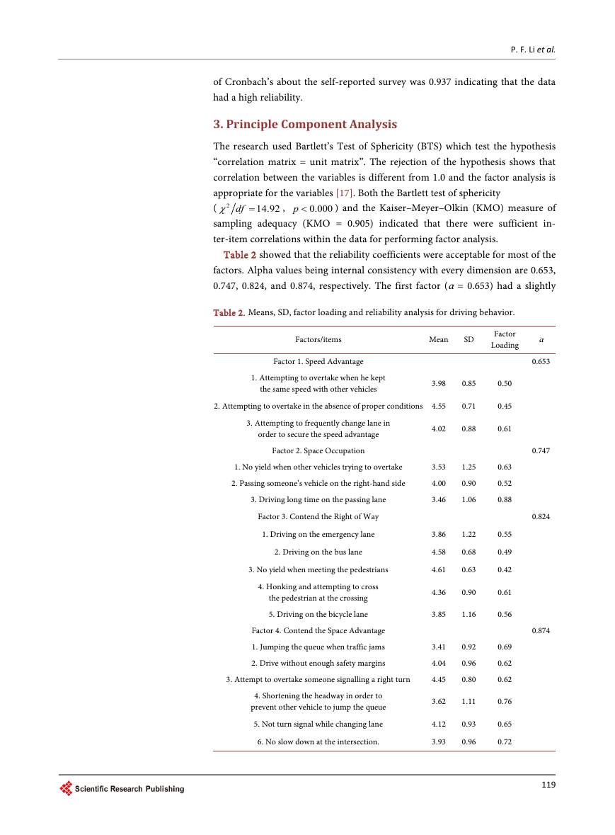
(1) The driver behavior self-reported survey consisted of 17 items (see Table
2). These questions concerning traffic matters were selected to cover violations
117
�
P. F. Li et al.
118
of the traffic code, vehicle interaction and the pedestrian-vehicle interaction.
Drivers were asked to indicate how often they carried out each of the activities.
The five point Likert scale applied ranged from “very often (mark 1)” to “never
(mark 5)”.
(2) Information was also gathered regarding respondents, including gender,
age, driving experience, driving time per week, whether the driver occurred in
traffic accidents within five years, and so on.
2.2. Participants
A questionnaire survey was carried out in May 2014 on the internet. 225 valid
questionnaires were received. All respondents were required to have a valid
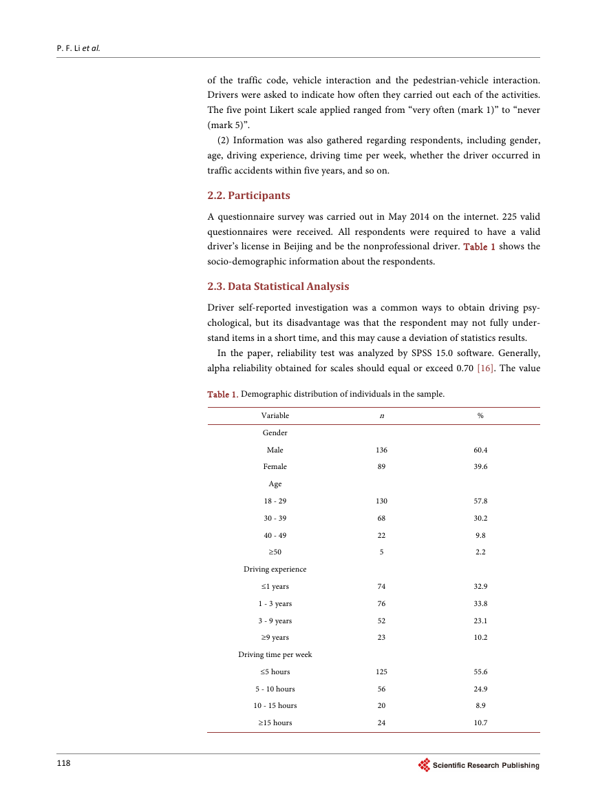
driver’s license in Beijing and be the nonprofessional driver. Table 1 shows the
socio-demographic information about the respondents.
2.3. Data Statistical Analysis
Driver self-reported investigation was a common ways to obtain driving psy-
chological, but its disadvantage was that the respondent may not fully under-
stand items in a short time, and this may cause a deviation of statistics results.
In the paper, reliability test was analyzed by SPSS 15.0 software. Generally,
alpha reliability obtained for scales should equal or exceed 0.70 [16]. The value
Table 1. Demographic distribution of individuals in the sample.
Variable
Gender
Male
Female
Age
18 - 29
30 - 39
40 - 49
≥50
Driving experience
≤1 years
1 - 3 years
3 - 9 years
≥9 years
Driving time per week
≤5 hours
5 - 10 hours
10 - 15 hours
≥15 hours
n
136
89
130
68
22
5
74
76
52
23
125
56
20
24
%
60.4
39.6
57.8
30.2
9.8
2.2
32.9
33.8
23.1
10.2
55.6
24.9
8.9
10.7
�
of Cronbach’s about the self-reported survey was 0.937 indicating that the data
had a high reliability.
P. F. Li et al.
3. Principle Component Analysis
The research used Bartlett’s Test of Sphericity (BTS) which test the hypothesis
“correlation matrix = unit matrix”. The rejection of the hypothesis shows that
correlation between the variables is different from 1.0 and the factor analysis is
appropriate for the variables [17]. Both the Bartlett test of sphericity
(
) and the Kaiser–Meyer–Olkin (KMO) measure of
dfχ
sampling adequacy (KMO = 0.905) indicated that there were sufficient in-
ter-item correlations within the data for performing factor analysis.
14.92
,
p <
0.000
2
=
Table 2 showed that the reliability coefficients were acceptable for most of the
factors. Alpha values being internal consistency with every dimension are 0.653,
0.747, 0.824, and 0.874, respectively. The first factor (α = 0.653) had a slightly
Table 2. Means, SD, factor loading and reliability analysis for driving behavior.
Factors/items
Mean
SD
Factor
Loading
α
Factor 1. Speed Advantage
0.653
1. Attempting to overtake when he kept
the same speed with other vehicles
3.98
0.85
2. Attempting to overtake in the absence of proper conditions 4.55
0.71
3. Attempting to frequently change lane in
order to secure the speed advantage
4.02
0.88
Factor 2. Space Occupation
1. No yield when other vehicles trying to overtake
2. Passing someone’s vehicle on the right-hand side
3. Driving long time on the passing lane
Factor 3. Contend the Right of Way
1. Driving on the emergency lane
2. Driving on the bus lane
3. No yield when meeting the pedestrians
4. Honking and attempting to cross
the pedestrian at the crossing
5. Driving on the bicycle lane
Factor 4. Contend the Space Advantage
1. Jumping the queue when traffic jams
2. Drive without enough safety margins
3. Attempt to overtake someone signalling a right turn
4. Shortening the headway in order to
prevent other vehicle to jump the queue
5. Not turn signal while changing lane
6. No slow down at the intersection.
3.53
4.00
3.46
3.86
4.58
4.61
1.25
0.90
1.06
1.22
0.68
0.63
4.36
0.90
3.85
1.16
3.41
4.04
4.45
0.92
0.96
0.80
3.62
1.11
4.12
3.93
0.93
0.96
0.50
0.45
0.61
0.63
0.52
0.88
0.55
0.49
0.42
0.61
0.56
0.69
0.62
0.62
0.76
0.65
0.72
0.747
0.824
0.874
119
�
P. F. Li et al.
lower a-value than 0.7. Others factors were greater than 0.7, and they were satis-
factory.
Principle component analysis with varimax rotation was used to extract fac-
tors. Eigenvalue was used to determine the number of factors extracted. The ini-
tial factor analysis result revealed a four-factor solution, which accounted for
66% of variance.
As shown in Table 2, the first factor was entitled speed advantage, such as at-
tempting to overtake when he kept the same speed with other vehicles, attempt-
ing to overtake in the absence of proper conditions and frequently change lane
in order to secure the speed advantage. The second factor, space occupation
means that the driver himself occupies a favorable position, and prevents the
other vehicle passing. It related to driving long time on the passing lane, no yield
when other vehicles trying to overtake, etc. Factor 3, contend the rights of way
indicates that the driver competes for the right of way with other traffic respon-
dents while driving. It included no yield, honking and attempting to cross the
pedestrian at the crossing, driving in the emergency/bus/bicycle lane. The last
factor, contend the space advantage means that the driver grabs the favorable
traffic position in traffic jams. It covered item related to jumping the queue
when traffic jams, driving without enough safety margins, shortening the head-
way in order to prevent other vehicle to jump the queue, and so on. Space occu-
pation and contend the space advantage have a different connotation. The for-
mer is to maintain its own favorable position; the latter is to grab the favorable
traffic position.
4. Driver Classification Based on the FCM
4.1. FCM
Advanced driver assistance systems need to adapt different strategies to different
groups of drivers. This paper quantified driver characteristics by confirmatory
factor analysis. The FCM algorithm which uses an iterative algorithm to deter-
mine the membership degree from each object to its cluster centroid over all
clusters by the membership function was selected to classify the drivers.
,
f
,
}
,
=
{
R
X
x
i
∈
x
n
x x
,
1
2
In this section, the FCM algorithm was briefly described. Consider a set of
unlabeled patterns
, where n is the number of pat-
terns and f is the dimension of pattern vectors (features). The FCM algorithm
focuses on minimizing the value of an objective function. The objective function
measures the quality of the partitioning that divides a dataset into C clusters.
The objective function is an optimization function that calculates the weighted
within-group sum of squared errors (WGSS) as follows:
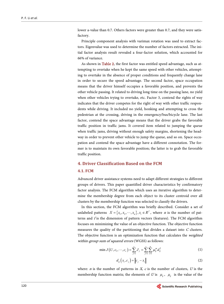
min
(
J U c
,
1
,
,
c
c
)
=
c
=∑
J
j
j
1
=
c
n
∑∑
j
1
=
i
1
=
m
dµ
ij
2
ij
(1)
(
d
ij
x c
,
i
j
)
=
c
j
−
x
i
(2)
where: n is the number of patterns in X, c is the number of clusters, U is the
membership function matrix; the elements of U is
ijµ is the value of the
ijµ ,
120
�
P. F. Li et al.
ijd is the dis-
membership function of the i pattern belonging to the j cluster,
tance from xi to cj, cj denotes the cluster center of the j cluster, m is the exponent
on
ijµ to control fuzziness or amount of clusters overlap.
The FCM algorithm subject to the following constraints on U:
c
∑
j
1
=
µ
ij
=
1,
i
=
1, 2,
(3)
n
,
Function (1) describes a constrained optimization problem, which can be
converted to an unconstrained optimization problem by using the Lagrange
multiplier technique.
c
j
=
n
∑
i
1
=
n
∑
i
1
=
m
µ
ij
x
i
m
µ
ij
(4)
µ
ij
=
c
∑
k
1
=
1
ij
kj
d
d
(5)
2
(
m
)
1
−
The FCM algorithm starts with a set of initial cluster centers (or arbitrary
membership values). Then, it iterates the two updating functions (4) and (5) un-
til the cluster centers are stable or the objective function in (1) converges to a
local minimum. The complete algorithm consists of the following steps:
Step 1: Given a fixed number C, initialize the cluster center matrix U0 by using
a random generator from the original dataset. Record the cluster centers, set k =
0, m = 2, and decide ε , where ε is a small positive constant.
Step 2: Initialize the membership matrix U0 by functions (5).
Step 3: Compute the new cluster center matrix (candidate) cj by (4).
Step 4: Compute the new membership matrix Uk by (5).
Step 5: if
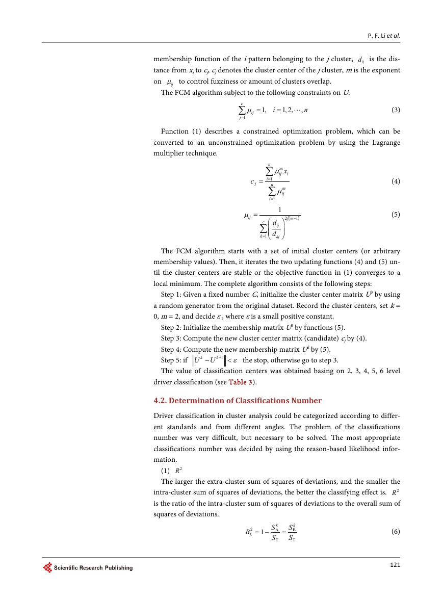
The value of classification centers was obtained basing on 2, 3, 4, 5, 6 level
< the stop, otherwise go to step 3.
U U
1
ε−
−
k
k
driver classification (see Table 3).
4.2. Determination of Classifications Number
Driver classification in cluster analysis could be categorized according to differ-
ent standards and from different angles. The problem of the classifications
number was very difficult, but necessary to be solved. The most appropriate
classifications number was decided by using the reason-based likelihood infor-
mation.
2R
(1)
The larger the extra-cluster sum of squares of deviations, and the smaller the
2R
intra-cluster sum of squares of deviations, the better the classifying effect is.
is the ratio of the intra-cluster sum of squares of deviations to the overall sum of
squares of deviations.
2
R
k
= −
1
k
S
A
S
T
=
S
S
k
B
T
(6)
121
�
P. F. Li et al.
Table 3. Values of significant influence factors classification centers
Type A
Type B
Type A
Type B
Type C
Type A
Type B
Type C
Type D
Type A
Type B
Type C
Type D
Type E
Type A
Type B
Type C
Type D
Type E
Type F
Factor 1
Factor 2
Factor 3
Factor 4
4.603
3.666
4.773
4.198
3.461
4.840
4.320
4.035
3.396
4.860
4.357
4.156
3.567
2.929
4.892
4.432
4.175
4.121
3.540
2.889
4.386
3.087
4.626
3.702
2.897
4.714
4.070
3.300
2.842
4.743
4.129
3.365
2.901
3.002
4.794
4.028
4.177
3.267
2.836
2.993
4.733
4.099
4.843
4.467
3.959
4.889
4.534
4.336
3.906
4.902
4.548
4.413
4.170
3.044
4.921
4.595
4.503
4.368
4.151
2.947
4.517
3.465
4.730
4.021
3.249
4.818
4.137
3.879
3.173
4.841
4.177
4.008
3.336
2.743
4.875
4.368
3.855
3.984
3.307
2.695
S
k
A
=
k
∑
k
1
=
(
W k
)
=
k m
∑∑ ∑
1 n
=
l
j
S
∈
1
=
n
k
i
(
n
n
l µ
j
i
−
)2
(7)
S
T
=
m
∑ ∑
1 n
=
l
j
S
∈
n
i
(
n
n
l µ
j
i
−
)2
(8)
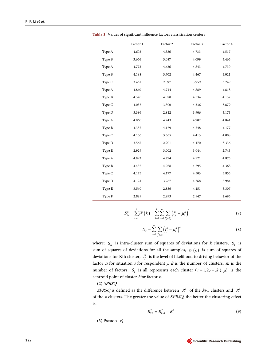
AS is intra-cluster sum of squares of deviations for k clusters,
TS is
where:
)W k is sum of squares of
sum of squares of deviations for all the samples,
n
jl is the level of likelihood to driving behavior of the
deviations for Kth cluster,
factor n for situation i for respondent j, k is the number of clusters, m is the
number of factors,
iµ is the
n
centroid point of cluster i for factor n.
iS is all represents each cluster (
= ),
1, 2,
k
(
i
,
(2) SPRSQ
SPRSQ is defined as the difference between
2R
of the k clusters. The greater the value of SPRSQ, the better the clustering effect
is.
2R of the k+1 clusters and
(3) Pseudo
PF
2
R
SP
=
2
R
1k
+
−
2
R
k
(9)
122
�


 2023年江西萍乡中考道德与法治真题及答案.doc
 2012年重庆南川中考生物真题及答案.doc
 2013年江西师范大学地理学综合及文艺理论基础考研真题.doc
 2020年四川甘孜小升初语文真题及答案I卷.doc
 2020年注册岩土工程师专业基础考试真题及答案.doc
 2023-2024学年福建省厦门市九年级上学期数学月考试题及答案.doc
 2021-2022学年辽宁省沈阳市大东区九年级上学期语文期末试题及答案.doc
 2022-2023学年北京东城区初三第一学期物理期末试卷及答案.doc
 2018上半年江西教师资格初中地理学科知识与教学能力真题及答案.doc
 2012年河北国家公务员申论考试真题及答案-省级.doc
 2020-2021学年江苏省扬州市江都区邵樊片九年级上学期数学第一次质量检测试题及答案.doc
 2022下半年黑龙江教师资格证中学综合素质真题及答案.doc