An Introduction
to Restricted Boltzmann Machines
Asja Fischer1,2 and Christian Igel2
1 Institut f¨ur Neuroinformatik, Ruhr-Universit¨at Bochum, Germany
2 Department of Computer Science, University of Copenhagen, Denmark
Abstract. Restricted Boltzmann machines (RBMs) are probabilistic
graphical models that can be interpreted as stochastic neural networks.
The increase in computational power and the development of faster learn-
ing algorithms have made them applicable to relevant machine learning
problems. They attracted much attention recently after being proposed
as building blocks of multi-layer learning systems called deep belief net-
works. This tutorial introduces RBMs as undirected graphical models.
The basic concepts of graphical models are introduced first, however,
basic knowledge in statistics is presumed. Different learning algorithms
for RBMs are discussed. As most of them are based on Markov chain
Monte Carlo (MCMC) methods, an introduction to Markov chains and
the required MCMC techniques is provided.
1
Introduction
Boltzmann machines (BMs) have been introduced as bidirectionally connected
networks of stochastic processing units, which can be interpreted as neural net-
work models [1,16]. A BM can be used to learn important aspects of an unknown
probability distribution based on samples from this distribution. In general, this
learning process is difficult and time-consuming. However, the learning problem
can be simplified by imposing restrictions on the network topology, which leads
us to restricted Boltzmann machines (RBMs, [34]), the topic of this tutorial.
A (restricted) BM is a parameterized generative model representing a prob-
ability distribution. Given some observations, the training data, learning a BM
means adjusting the BM parameters such that the probability distribution repre-
sented by the BM fits the training data as well as possible. Boltzmann machines
consist of two types of units, so called visible and hidden neurons, which can be
thought of as being arranged in two layers. The visible units constitute the first
layer and correspond to the components of an observation (e.g., one visible unit
for each pixel of a digital input image). The hidden units model dependencies
between the components of observations (e.g., dependencies between pixels in
images). They can be viewed as non-linear feature detectors [16].
Boltzmann machines can also be regarded as particular graphical models [22],
more precisely undirected graphical models also known as Markov random fields.
The embedding of BMs into the framework of probabilistic graphical models
provides immediate access to a wealth of theoretical results and well-developed
L. Alvarez et al. (Eds.): CIARP 2012, LNCS 7441, pp. 14–36, 2012.
c Springer-Verlag Berlin Heidelberg 2012
�
An Introduction to Restricted Boltzmann Machines
15
algorithms. Therefore, our tutorial introduces RBMs from this perspective. Com-
puting the likelihood of an undirected model or its gradient for inference is in
general computationally intensive, and this also holds for RBMs. Thus, sampling
based methods are employed to approximate the likelihood and its gradient.
Sampling from an undirected graphical model is in general not straightforward,
but for RBMs Markov chain Monte Carlo (MCMC) methods are easily appli-
cable in the form of Gibbs sampling, which will be introduced in this tutorial
along with basic concepts of Markov chain theory.
After successful learning, an RBM provides a closed-form representation of
the distribution underlying the observations. It can be used to compare the
probabilities of (unseen) observations and to sample from the learnt distribution
(e.g., to generate image textures [25,21]), in particular from marginal distribu-
tions of interest. For example, we can fix some visible units corresponding to a
partial observation and sample the remaining visible units for completing the
observation (e.g., to solve an image inpainting task [21]).
Boltzmann machines have been proposed in the 1980s [1,34]. Compared to
the times when they were first introduced, RBMs can now be applied to more
interesting problems due to the increase in computational power and the de-
velopment of new learning strategies [15]. Restricted Boltzmann machines have
received a lot of attention recently after being proposed as building blocks of
multi-layer learning architectures called deep belief networks (DBNs, [19,17]).
The idea is that the hidden neurons extract relevant features from the observa-
tions. These features can serve as input to another RBM. By stacking RBMs in
this way, one can learn features from features in the hope of arriving at a high
level representation.
It is an important property that single as well as stacked RBMs can be rein-
terpreted as deterministic feed-forward neural networks. Than they are used as
functions from the domain of the observations to the expectations of the la-
tent variables in the top layer. Such a function maps the observations to learnt
features, which can, for example, serve as input to a supervised learning sys-
tem. Further, the neural network corresponding to a trained RBM or DBN can
be augmented by an output layer, where units in the new added output layer
represent labels corresponding to observations. Then the model corresponds to
a standard neural network for classification or regression that can be further
trained by standard supervised learning algorithms [31]. It has been argued that
this initialization (or unsupervised pretraining) of the feed-forward neural net-
work weights based on a generative model helps to overcome problems observed
when training multi-layer neural networks [19].
This introduction to RBMs is meant to supplement existing tutorials, such as
the highly recommended review by Bengio [2], by providing more background
information on Markov random fields and MCMC methods in Section 2 and
Section 3, respectively. However, basic knowledge in statistics is presumed. We
put an emphasis on topics that are – based on our experience – sometimes not
familiar to people starting with RBMs. Restricted Boltzmann machines will be
presented in Section 4. Section 5 will consider RBM training algorithms based
�
16
A. Fischer and C. Igel
on approximations of the log-likelihood gradient. This includes a discussion of
contrastive divergence learning [15] as well as parallel tempering [10]. We will
close by hinting at generalizations of RBMs in sections 6 and 7.
2 Graphical Models
Probabilistic graphical models describe probability distributions by mapping
conditional dependence and independence properties between random variables
on a graph structure (two sets of random variables X 1 and X 2 are condi-
tionally independent given a set of random variables X 3 if p(X 1, X 2|X 3) =
p(X 1|X 3)p(X 2|X 3)). Visualization by graphs can help to develop, understand
and motivate probabilistic models. Furthermore, complex computations (e.g.,
marginalization) can be derived efficiently by using algorithms exploiting the
graph structure.
There exist graphical models associated with different kind of graph struc-
tures, for example factor graphs, Bayesian networks associated with directed
graphs, and Markov random fields, which are also called Markov networks or
undirected graphical models. This tutorial focuses on the latter. A general in-
troduction to graphical models for machine learning can, for example be found
in [5]. The most comprehensive resource on graphical models is the textbook by
Koller and Friedman [22].
2.1 Undirected Graphs and Markov Random Fields
First, we will summarize some fundamental concepts from graph theory. An
undirected graph is a tuple G = (V, E), where V is a finite set of nodes and E is
a set of undirected edges. An edge consists out of a pair of nodes from V . If there
exists an edge between two nodes v and w, i.e. {v, w} ∈ E, w belongs to the
neighborhood of v and vice versa. The neighborhood Nv := {w ∈ V : {w, v} ∈ E}
of v is defined by the set of nodes connected to v. A clique is a subset of V in
which all nodes are pairwise connected. A clique is called maximal if no node
can be added such that the resulting set is still a clique. In the following we will
denote by C the set of all maximal cliques of an undirected graph. We call a
sequence of nodes v1, v2, . . . , vm ∈ V , with {vi, vi+1} ∈ E for i = 1, . . . , m − 1 a
path from v1 to vm. A set V ⊂ V separates two nodes v /∈ V and w /∈ V, if every
path from v to w contains a node from V.
We now associate a random variable Xv taking values in a state space Λv
with each node v in an undirected graph G = (V, E). To ease the notation, we
assume Λv = Λ for all v ∈ V . The random variables X = (Xv)v∈V are called
Markov random field (MRF) if the joint probability distribution p fulfills the
(global) Markov property w.r.t. the graph: For all disjunct subsets A,B,S ⊂ V ,
where all nodes in A and B are separated by S the variables (Xa)a∈A and
(Xb)b∈B are conditional independent given (Xs)s∈S, i.e. for all x ∈ Λ
it holds
p ((xa)a∈A|(xt)t∈S∪B) = p ((xa)a∈A|(xt)t∈S). A set of nodes MB(v) is called
the Markov blanket of node v, if for any set of nodes B with v ∈ B we have
|V |
�
An Introduction to Restricted Boltzmann Machines
17
p(v | MB(v),B) = p(v | MB(v)). This means that v is conditional independent
from any other variables given MB(v). In an MRF, the Markov blanket MB(v) is
given by the neighborhood Nv of v, a fact that is also referred to as local Markov
property.
Since conditional independence of random variables and the factorization
properties of the joint probability distribution are closely related, one can ask
if there exists a general factorization form of the distributions of MRFs. An an-
swer to this question is given by the Hammersley-Clifford Theorem (for rigorous
formulations and proofs we refer to [23,22]). The theorem states that a strictly
positive distribution p satisfies the Markov property w.r.t. an undirected graph
G if and only if p factorizes over G. A distribution is said to factorize about an
undirected graph G with maximal cliques C if there exists a set of non-negative
functions {ψC}C⊂C, called potential functions, with
∀x, ˆx ∈ Λ
|V |
and
: (xc)c∈C = (ˆxc)c∈C ⇒ ψC (x) = ψC (ˆx)
p(x) =
1
Z
ψC (x).
(1)
(2)
(3)
The normalization constant Z =
C∈C
C∈C ψC (xC ) is called partition function.
If p is strictly positive, the same holds for the potential functions. Thus we
can write
x
p(x) =
ψC (xC ) =
C∈C ln ψC (xC ) =
1
Z
e
−E(x) ,
e
1
Z
C∈C
1
Z
C∈C ln ψC (xC) the energy function. Thus, the probability
where we call E :=
distribution of every MRF can be expressed in the form given by (3), which is
also called Gibbs distribution.
2.2 Unsupervised Learning
Unsupervised learning means learning (important aspects of) an unknown dis-
tribution q based on sample data. This includes finding new representations of
data that foster learning, generalization, and communication. If we assume that
the structure of the graphical model is known and the energy function belongs to
a known family of functions parameterized by θ, unsupervised learning of a data
distribution with an MRF means adjusting the parameters θ. We write p(x|θ)
when we want to emphasize the dependency of a distribution on its parameters.
We consider training data S = {x1, . . . , x}. The data samples are assumed
to be independent and identically distributed (i.i.d.). That is, they are drawn
independently from some unknown distribution q. A standard way of estimating
the parameters of a statistical model is maximum-likelihood estimation. Applied
to MRFs, this corresponds to finding the MRF parameters that maximize the
probability of S under the MRF distribution, i.e. training corresponds to finding
the parameters θ that maximize the likelihood given the training data. The
�
18
A. Fischer and C. Igel
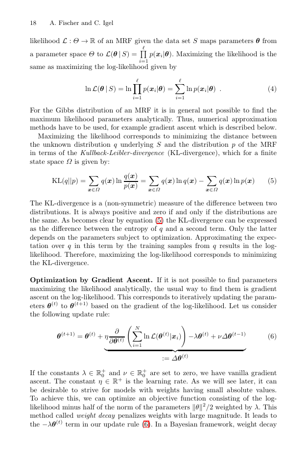
likelihood L : Θ → R of an MRF given the data set S maps parameters θ from
a parameter space Θ to L(θ | S) =
p(xi|θ). Maximizing the likelihood is the
same as maximizing the log-likelihood given by
i=1
lnL(θ | S) = ln
p(xi|θ) =
ln p(xi|θ) .
(4)
i=1
i=1
For the Gibbs distribution of an MRF it is in general not possible to find the
maximum likelihood parameters analytically. Thus, numerical approximation
methods have to be used, for example gradient ascent which is described below.
Maximizing the likelihood corresponds to minimizing the distance between
the unknown distribution q underlying S and the distribution p of the MRF
in terms of the Kullback-Leibler-divergence (KL-divergence), which for a finite
state space Ω is given by:
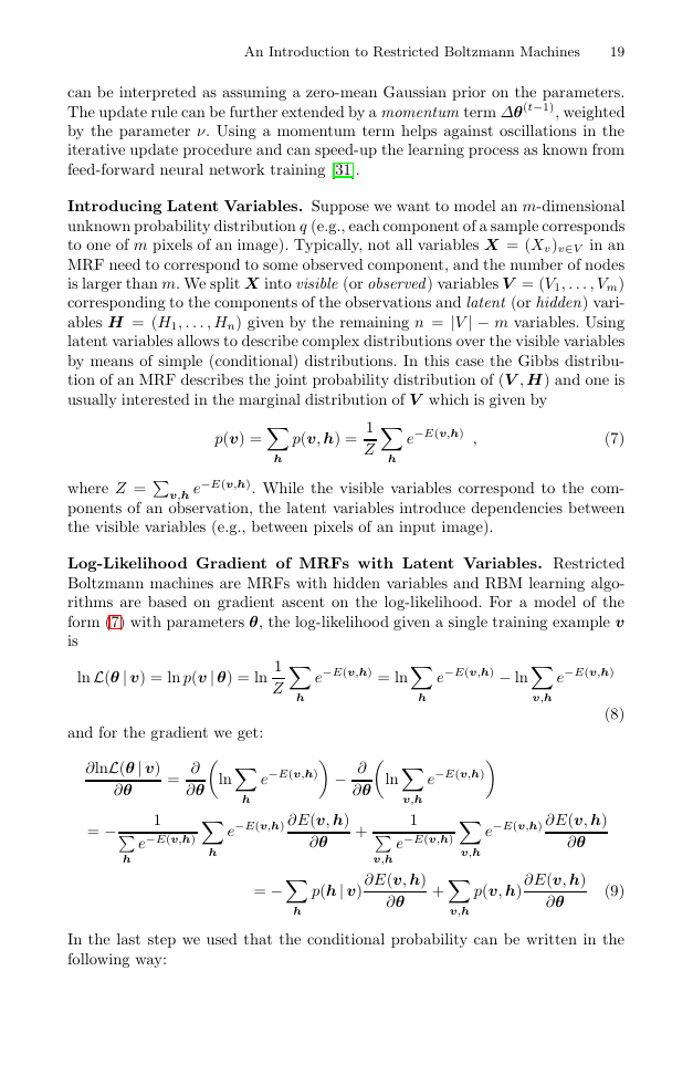
KL(q||p) =
q(x) ln
q(x)
p(x)
=
q(x) ln q(x) −
q(x) ln p(x)
(5)
x∈Ω
x∈Ω
x∈Ω
The KL-divergence is a (non-symmetric) measure of the difference between two
distributions. It is always positive and zero if and only if the distributions are
the same. As becomes clear by equation (5) the KL-divergence can be expressed
as the difference between the entropy of q and a second term. Only the latter
depends on the parameters subject to optimization. Approximating the expec-
tation over q in this term by the training samples from q results in the log-
likelihood. Therefore, maximizing the log-likelihood corresponds to minimizing
the KL-divergence.
N
lnL(θ(t)|xi)
Optimization by Gradient Ascent. If it is not possible to find parameters
maximizing the likelihood analytically, the usual way to find them is gradient
ascent on the log-likelihood. This corresponds to iteratively updating the param-
eters θ(t) to θ(t+1) based on the gradient of the log-likelihood. Let us consider
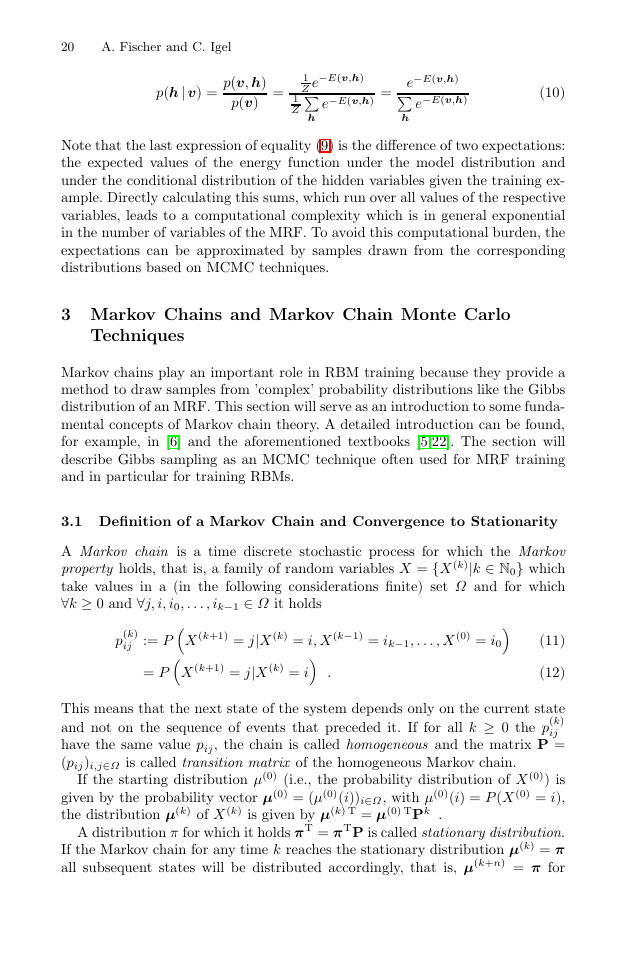
the following update rule:
∂
i=1
∂θ(t)
θ(t+1) = θ(t) + η
−λθ(t) + νΔθ(t−1)
If the constants λ ∈ R+
0 and ν ∈ R+
0 are set to zero, we have vanilla gradient
ascent. The constant η ∈ R+ is the learning rate. As we will see later, it can
be desirable to strive for models with weights having small absolute values.
To achieve this, we can optimize an objective function consisting of the log-
likelihood minus half of the norm of the parameters θ2/2 weighted by λ. This
method called weight decay penalizes weights with large magnitude. It leads to
the −λθ(t) term in our update rule (6). In a Bayesian framework, weight decay
:= Δθ(t)
(6)
�
An Introduction to Restricted Boltzmann Machines
19
can be interpreted as assuming a zero-mean Gaussian prior on the parameters.
The update rule can be further extended by a momentum term Δθ(t−1), weighted
by the parameter ν. Using a momentum term helps against oscillations in the
iterative update procedure and can speed-up the learning process as known from
feed-forward neural network training [31].
Introducing Latent Variables. Suppose we want to model an m-dimensional
unknown probability distribution q (e.g., each component of a sample corresponds
to one of m pixels of an image). Typically, not all variables X = (Xv)v∈V in an
MRF need to correspond to some observed component, and the number of nodes
is larger than m. We split X into visible (or observed ) variables V = (V1, . . . , Vm)
corresponding to the components of the observations and latent (or hidden) vari-
ables H = (H1, . . . , Hn) given by the remaining n = |V | − m variables. Using
latent variables allows to describe complex distributions over the visible variables
by means of simple (conditional) distributions. In this case the Gibbs distribu-
tion of an MRF describes the joint probability distribution of (V , H) and one is
usually interested in the marginal distribution of V which is given by
h
1
Z
p(v) =
p(v, h) =
h
−E(v,h) ,
e
(7)
−E(v,h). While the visible variables correspond to the com-
where Z =
ponents of an observation, the latent variables introduce dependencies between
the visible variables (e.g., between pixels of an input image).
v,h e
Log-Likelihood Gradient of MRFs with Latent Variables. Restricted
Boltzmann machines are MRFs with hidden variables and RBM learning algo-
rithms are based on gradient ascent on the log-likelihood. For a model of the
form (7) with parameters θ, the log-likelihood given a single training example v
is
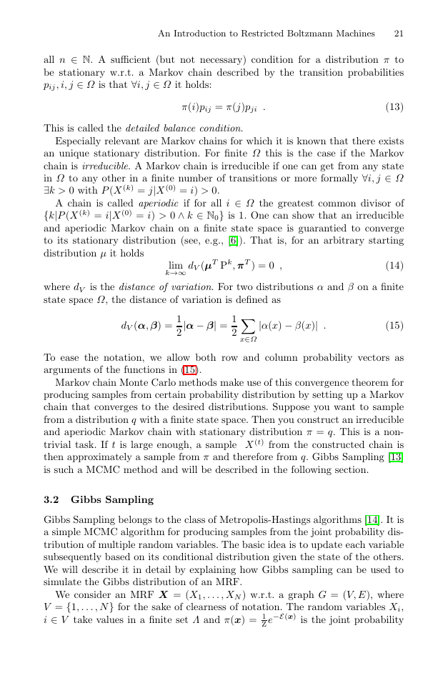
lnL(θ | v) = ln p(v | θ) = ln
and for the gradient we get:
−E(v,h) − ln
−E(v,h) = ln
−E(v,h)
1
Z
e
h
e
h
(8)
e
v,h
∂lnL(θ | v)
1
∂θ
= −
=
∂
∂θ
−E(v,h)
ln
e
− ∂
∂θ
h
−E(v,h) ∂E(v, h)
e−E(v,h)
e
h
h
1
v,h
ln
v,h
−E(v,h)
e
v,h
∂θ
+
e−E(v,h)
e
−E(v,h) ∂E(v, h)
∂θ
= −
p(h| v)
∂E(v, h)
∂θ
+
p(v, h)
v,h
∂E(v, h)
∂θ
(9)
h
In the last step we used that the conditional probability can be written in the
following way:
�
20
A. Fischer and C. Igel
p(h| v) =
p(v, h)
p(v)
=
1
Z
1
Z e
h
−E(v,h)
e−E(v,h)
e
h
=
−E(v,h)
e−E(v,h)
(10)
Note that the last expression of equality (9) is the difference of two expectations:
the expected values of the energy function under the model distribution and
under the conditional distribution of the hidden variables given the training ex-
ample. Directly calculating this sums, which run over all values of the respective
variables, leads to a computational complexity which is in general exponential
in the number of variables of the MRF. To avoid this computational burden, the
expectations can be approximated by samples drawn from the corresponding
distributions based on MCMC techniques.
3 Markov Chains and Markov Chain Monte Carlo
Techniques
Markov chains play an important role in RBM training because they provide a
method to draw samples from ’complex’ probability distributions like the Gibbs
distribution of an MRF. This section will serve as an introduction to some funda-
mental concepts of Markov chain theory. A detailed introduction can be found,
for example, in [6] and the aforementioned textbooks [5,22]. The section will
describe Gibbs sampling as an MCMC technique often used for MRF training
and in particular for training RBMs.
3.1 Definition of a Markov Chain and Convergence to Stationarity
A Markov chain is a time discrete stochastic process for which the Markov
take values in a (in the following considerations finite) set Ω and for which
property holds, that is, a family of random variables X = {X (k)|k ∈ N0} which
∀k ≥ 0 and ∀j, i, i0, . . . , ik−1 ∈ Ω it holds
X (k+1) = j|X (k) = i, X (k−1) = ik−1, . . . , X (0) = i0
X (k+1) = j|X (k) = i
p(k)
ij
:= P
(11)
(12)
= P
.
This means that the next state of the system depends only on the current state
and not on the sequence of events that preceded it. If for all k ≥ 0 the p(k)
ij
have the same value pij, the chain is called homogeneous and the matrix P =
(pij)i,j∈Ω is called transition matrix of the homogeneous Markov chain.
If the starting distribution μ(0) (i.e., the probability distribution of X (0)) is
given by the probability vector μ(0) = (μ(0)(i))i∈Ω, with μ(0)(i) = P (X (0) = i),
the distribution μ(k) of X (k) is given by μ(k) T = μ(0) TPk .
A distribution π for which it holds πT = πTP is called stationary distribution.
If the Markov chain for any time k reaches the stationary distribution μ(k) = π
all subsequent states will be distributed accordingly, that is, μ(k+n) = π for
�
An Introduction to Restricted Boltzmann Machines
21
all n ∈ N. A sufficient (but not necessary) condition for a distribution π to
be stationary w.r.t. a Markov chain described by the transition probabilities
pij, i, j ∈ Ω is that ∀i, j ∈ Ω it holds:
π(i)pij = π(j)pji .
(13)
This is called the detailed balance condition.
Especially relevant are Markov chains for which it is known that there exists
an unique stationary distribution. For finite Ω this is the case if the Markov
chain is irreducible. A Markov chain is irreducible if one can get from any state
in Ω to any other in a finite number of transitions or more formally ∀i, j ∈ Ω
∃k > 0 with P (X (k) = j|X (0) = i) > 0.
A chain is called aperiodic if for all i ∈ Ω the greatest common divisor of
{k|P (X (k) = i|X (0) = i) > 0 ∧ k ∈ N0} is 1. One can show that an irreducible
and aperiodic Markov chain on a finite state space is guarantied to converge
to its stationary distribution (see, e.g., [6]). That is, for an arbitrary starting
distribution μ it holds
k→∞ dV (μT Pk, πT ) = 0 ,
lim
(14)
where dV is the distance of variation. For two distributions α and β on a finite
state space Ω, the distance of variation is defined as
x∈Ω
dV (α, β) =
|α − β| =
1
2
1
2
|α(x) − β(x)| .
(15)
To ease the notation, we allow both row and column probability vectors as
arguments of the functions in (15).
Markov chain Monte Carlo methods make use of this convergence theorem for
producing samples from certain probability distribution by setting up a Markov
chain that converges to the desired distributions. Suppose you want to sample
from a distribution q with a finite state space. Then you construct an irreducible
and aperiodic Markov chain with stationary distribution π = q. This is a non-
trivial task. If t is large enough, a sample X (t) from the constructed chain is
then approximately a sample from π and therefore from q. Gibbs Sampling [13]
is such a MCMC method and will be described in the following section.
3.2 Gibbs Sampling
Gibbs Sampling belongs to the class of Metropolis-Hastings algorithms [14]. It is
a simple MCMC algorithm for producing samples from the joint probability dis-
tribution of multiple random variables. The basic idea is to update each variable
subsequently based on its conditional distribution given the state of the others.
We will describe it in detail by explaining how Gibbs sampling can be used to
simulate the Gibbs distribution of an MRF.
We consider an MRF X = (X1, . . . , XN ) w.r.t. a graph G = (V, E), where
V = {1, . . . , N} for the sake of clearness of notation. The random variables Xi,
i ∈ V take values in a finite set Λ and π(x) = 1
−E(x) is the joint probability
Z e
�


 2023年江西萍乡中考道德与法治真题及答案.doc
 2012年重庆南川中考生物真题及答案.doc
 2013年江西师范大学地理学综合及文艺理论基础考研真题.doc
 2020年四川甘孜小升初语文真题及答案I卷.doc
 2020年注册岩土工程师专业基础考试真题及答案.doc
 2023-2024学年福建省厦门市九年级上学期数学月考试题及答案.doc
 2021-2022学年辽宁省沈阳市大东区九年级上学期语文期末试题及答案.doc
 2022-2023学年北京东城区初三第一学期物理期末试卷及答案.doc
 2018上半年江西教师资格初中地理学科知识与教学能力真题及答案.doc
 2012年河北国家公务员申论考试真题及答案-省级.doc
 2020-2021学年江苏省扬州市江都区邵樊片九年级上学期数学第一次质量检测试题及答案.doc
 2022下半年黑龙江教师资格证中学综合素质真题及答案.doc