A FAST ELITIST MULTIOBJECTIVE GENETIC ALGORITHM: NSGA-II ARAVIND SESHADRI 1. Multi-Objective Optimization Using NSGA-II NSGA ( [5]) is a popular non-domination based genetic algorithm for multi- It is a very effective algorithm but has been generally objective optimization. criticized for its computational complexity, lack of elitism and for choosing the optimal parameter value for sharing parameter σshare. A modified version, NSGA- II ( [3]) was developed, which has a better sorting algorithm , incorporates elitism and no sharing parameter needs to be chosen a priori. NSGA-II is discussed in detail in this. 2. 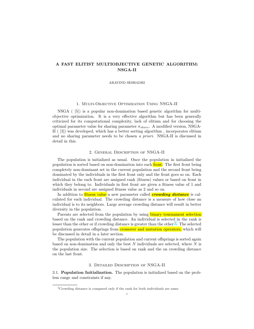General Description of NSGA-II The population is initialized as usual. Once the population in initialized the population is sorted based on non-domination into each front. The first front being completely non-dominant set in the current population and the second front being dominated by the individuals in the first front only and the front goes so on. Each individual in the each front are assigned rank (fitness) values or based on front in which they belong to. Individuals in first front are given a fitness value of 1 and individuals in second are assigned fitness value as 2 and so on. In addition to fitness value a new parameter called crowding distance is cal- culated for each individual. The crowding distance is a measure of how close an individual is to its neighbors. Large average crowding distance will result in better diversity in the population. Parents are selected from the population by using binary tournament selection based on the rank and crowding distance. An individual is selected in the rank is lesser than the other or if crowding distance is greater than the other 1. The selected population generates offsprings from crossover and mutation operators, which will be discussed in detail in a later section. The population with the current population and current offsprings is sorted again based on non-domination and only the best N individuals are selected, where N is the population size. The selection is based on rank and the on crowding distance on the last front. 3. Detailed Description of NSGA-II 3.1. Population Initialization. The population is initialized based on the prob- lem range and constraints if any. 1Crowding distance is compared only if the rank for both individuals are same 1 

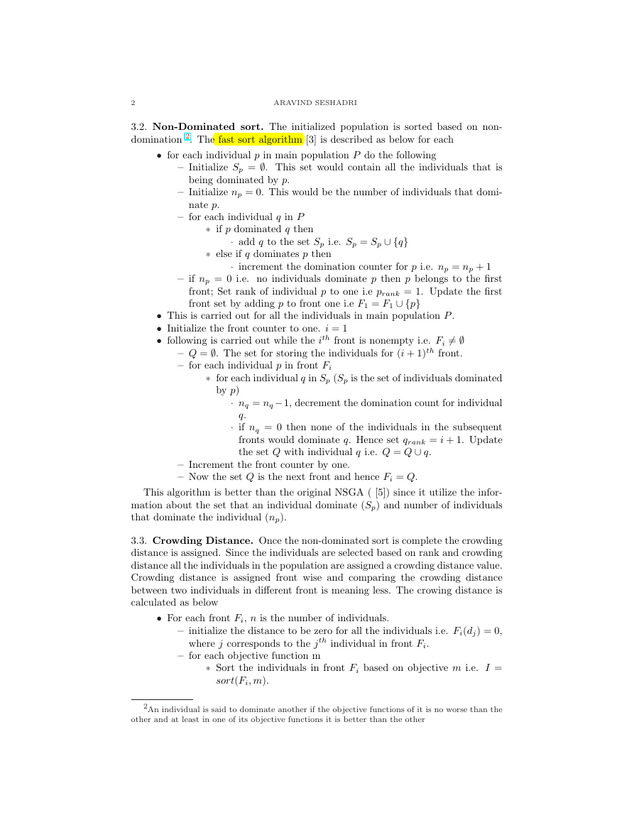
2 ARAVIND SESHADRI 3.2. Non-Dominated sort. The initialized population is sorted based on non- domination 2. The fast sort algorithm [3] is described as below for each • for each individual p in main population P do the following – Initialize Sp = ∅. This set would contain all the individuals that is – Initialize np = 0. This would be the number of individuals that domi- being dominated by p. nate p. – for each individual q in P ∗ if p dominated q then ∗ else if q dominates p then · add q to the set Sp i.e. Sp = Sp ∪ {q} · increment the domination counter for p i.e. np = np + 1 – if np = 0 i.e. no individuals dominate p then p belongs to the first front; Set rank of individual p to one i.e prank = 1. Update the first front set by adding p to front one i.e F1 = F1 ∪ {p} • This is carried out for all the individuals in main population P . • Initialize the front counter to one. i = 1 • following is carried out while the ith front is nonempty i.e. Fi = ∅ – Q = ∅. The set for storing the individuals for (i + 1)th front. – for each individual p in front Fi by p) ∗ for each individual q in Sp (Sp is the set of individuals dominated · nq = nq−1, decrement the domination count for individual q. · if nq = 0 then none of the individuals in the subsequent fronts would dominate q. Hence set qrank = i + 1. Update the set Q with individual q i.e. Q = Q ∪ q. – Increment the front counter by one. – Now the set Q is the next front and hence Fi = Q. This algorithm is better than the original NSGA ( [5]) since it utilize the infor- mation about the set that an individual dominate (Sp) and number of individuals that dominate the individual (np). 3.3. Crowding Distance. Once the non-dominated sort is complete the crowding distance is assigned. Since the individuals are selected based on rank and crowding distance all the individuals in the population are assigned a crowding distance value. Crowding distance is assigned front wise and comparing the crowding distance between two individuals in different front is meaning less. The crowing distance is calculated as below • For each front Fi, n is the number of individuals. – initialize the distance to be zero for all the individuals i.e. Fi(dj) = 0, where j corresponds to the jth individual in front Fi. – for each objective function m ∗ Sort the individuals in front Fi based on objective m i.e. I = sort(Fi, m). 2An individual is said to dominate another if the objective functions of it is no worse than the other and at least in one of its objective functions it is better than the other 

NSGA-II 3 ∗ Assign infinite distance to boundary values for each individual ∗ for k = 2 to (n − 1) in Fi i.e. I(d1) = ∞ and I(dn) = ∞ · I(dk) = I(dk) + I(k + 1).m − I(k − 1).m · I(k).m is the value of the mth objective function of the kth individual in I m − f min f max m The basic idea behind the crowing distance is finding the euclidian distance between each individual in a front based on their m objectives in the m dimensional hyper space. The individuals in the boundary are always selected since they have infinite distance assignment. 3.4. Selection. Once the individuals are sorted based on non-domination and with crowding distance assigned, the selection is carried out using a crowded- comparison-operator (≺n). The comparison is carried out as below based on (1) non-domination rank prank i.e. individuals in front Fi will have their rank as prank = i. (2) crowding distance Fi(dj) • p ≺n q if – prank < qrank – or if p and q belong to the same front Fi then Fi(dp) > Fi(dq) i.e. the crowing distance should be more. The individuals are selected by using a binary tournament selection with crowed- comparison-operator. 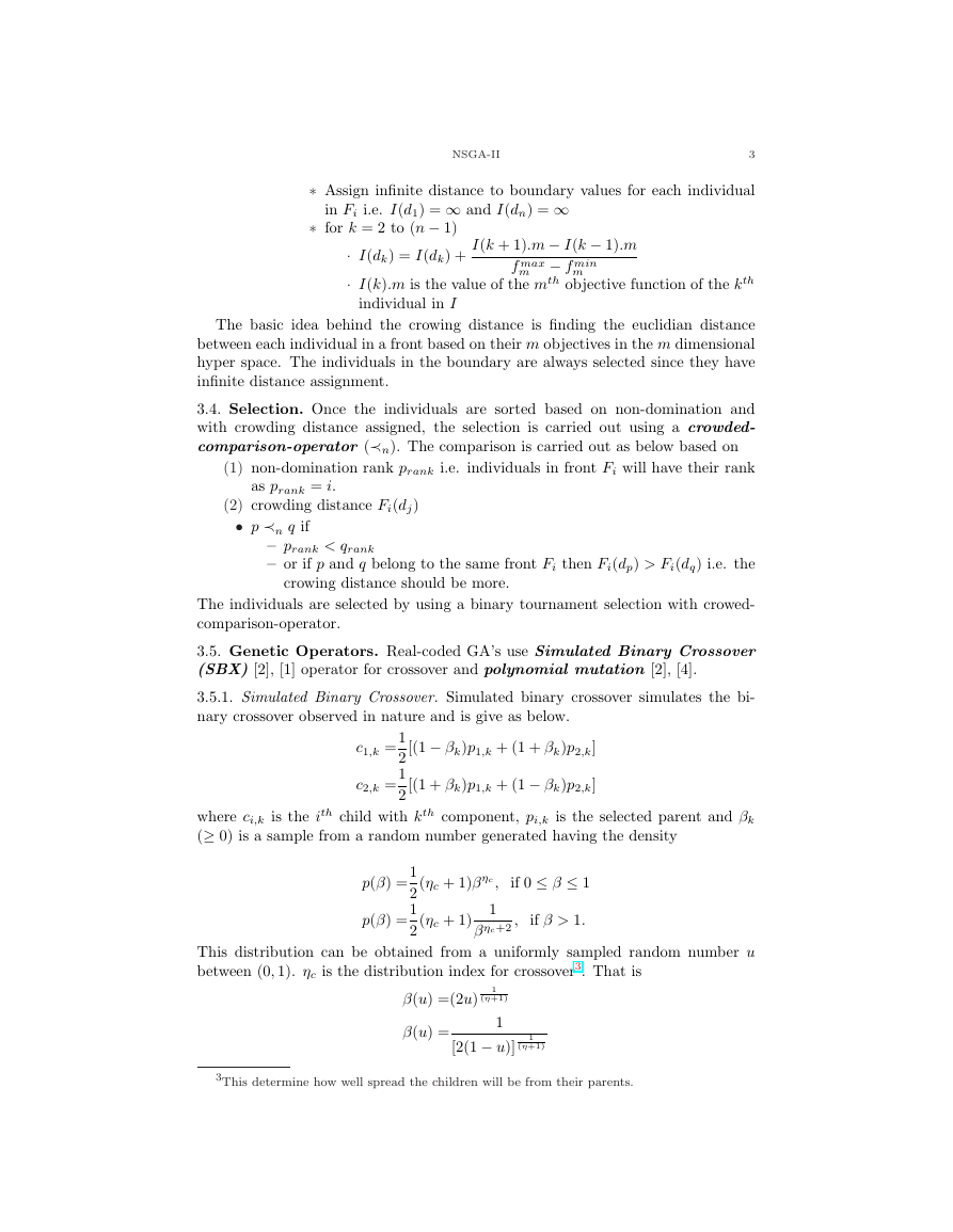3.5. Genetic Operators. Real-coded GA’s use Simulated Binary Crossover (SBX) [2], [1] operator for crossover and polynomial mutation [2], [4]. 3.5.1. Simulated Binary Crossover. Simulated binary crossover simulates the bi- nary crossover observed in nature and is give as below. c1,k = c2,k = 1 2 1 2 [(1 − βk)p1,k + (1 + βk)p2,k] [(1 + βk)p1,k + (1 − βk)p2,k] where ci,k is the ith child with kth component, pi,k is the selected parent and βk (≥ 0) is a sample from a random number generated having the density p(β) = p(β) = 1 2 1 2 (ηc + 1)βηc, 1 (ηc + 1) βηc+2 , if 0 ≤ β ≤ 1 if β > 1. This distribution can be obtained from a uniformly sampled random number u between (0, 1). ηc is the distribution index for crossover3. That is β(u) =(2u) 1 (η+1) β(u) = 1 [2(1 − u)] 1 (η+1) 3This determine how well spread the children will be from their parents. 

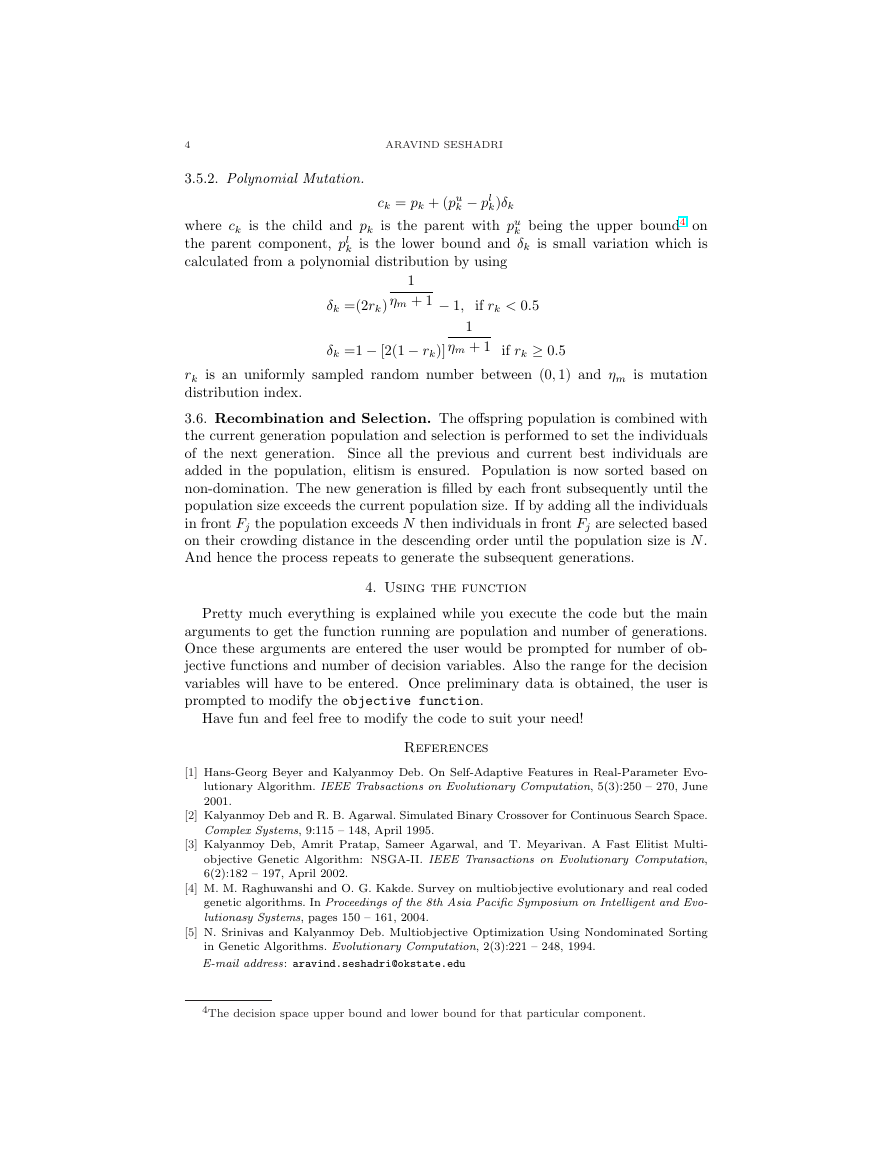
4 ARAVIND SESHADRI 3.5.2. Polynomial Mutation. k − pl k)δk where ck is the child and pk is the parent with pu the parent component, pl calculated from a polynomial distribution by using ck = pk + (pu k being the upper bound4 on k is the lower bound and δk is small variation which is 1 ηm + 1 − 1, δk =(2rk) if rk < 0.5 δk =1 − [2(1 − rk)] 1 ηm + 1 if rk ≥ 0.5 rk is an uniformly sampled random number between (0, 1) and ηm is mutation distribution index. 3.6. Recombination and Selection. The offspring population is combined with the current generation population and selection is performed to set the individuals of the next generation. Since all the previous and current best individuals are added in the population, elitism is ensured. Population is now sorted based on non-domination. The new generation is filled by each front subsequently until the population size exceeds the current population size. If by adding all the individuals in front Fj the population exceeds N then individuals in front Fj are selected based on their crowding distance in the descending order until the population size is N. And hence the process repeats to generate the subsequent generations. 4. Using the function Pretty much everything is explained while you execute the code but the main arguments to get the function running are population and number of generations. Once these arguments are entered the user would be prompted for number of ob- jective functions and number of decision variables. Also the range for the decision variables will have to be entered. Once preliminary data is obtained, the user is prompted to modify the objective function. Have fun and feel free to modify the code to suit your need! References [1] Hans-Georg Beyer and Kalyanmoy Deb. On Self-Adaptive Features in Real-Parameter Evo- lutionary Algorithm. IEEE Trabsactions on Evolutionary Computation, 5(3):250 – 270, June 2001. [2] Kalyanmoy Deb and R. B. Agarwal. Simulated Binary Crossover for Continuous Search Space. Complex Systems, 9:115 – 148, April 1995. [3] Kalyanmoy Deb, Amrit Pratap, Sameer Agarwal, and T. Meyarivan. A Fast Elitist Multi- objective Genetic Algorithm: NSGA-II. IEEE Transactions on Evolutionary Computation, 6(2):182 – 197, April 2002. [4] M. M. Raghuwanshi and O. G. Kakde. Survey on multiobjective evolutionary and real coded genetic algorithms. In Proceedings of the 8th Asia Pacific Symposium on Intelligent and Evo- lutionasy Systems, pages 150 – 161, 2004. [5] N. Srinivas and Kalyanmoy Deb. Multiobjective Optimization Using Nondominated Sorting in Genetic Algorithms. Evolutionary Computation, 2(3):221 – 248, 1994. E-mail address: aravind.seshadri@okstate.edu 4The decision space upper bound and lower bound for that particular component.