Smoothing of Pseudorange with Carrier Phase The idea behind the smoothing of pseudorange observations using integrated carrier phase observations (in short: code smoothing) has been elaborated by Mr. Ron Hatch in the beginning of the eighties (the smoothing algorithm is sometimes called the 'Hatch filter') and is based on the simple concept that the integrated carrier phase observation when converted to length unit ('carrier range') is also a measure of the range between an SV and a receiver, and the change in pseudorange between observations at different points of time (epochs) equals the change in carrier range. and the change in carrier range can be determined with far more accuracy (in practice in the order of mm's) than the change in pseodorange (in practice in the order of meters). Consider a series of N observations of N , to an SV: pseudoranges Pi and carrier ranges Ci , i = 1 , .. , epoch 1 ; P1 ; C1 epoch 2 ; P2 ; C2 etc etc epoch N ; PN ; CN. 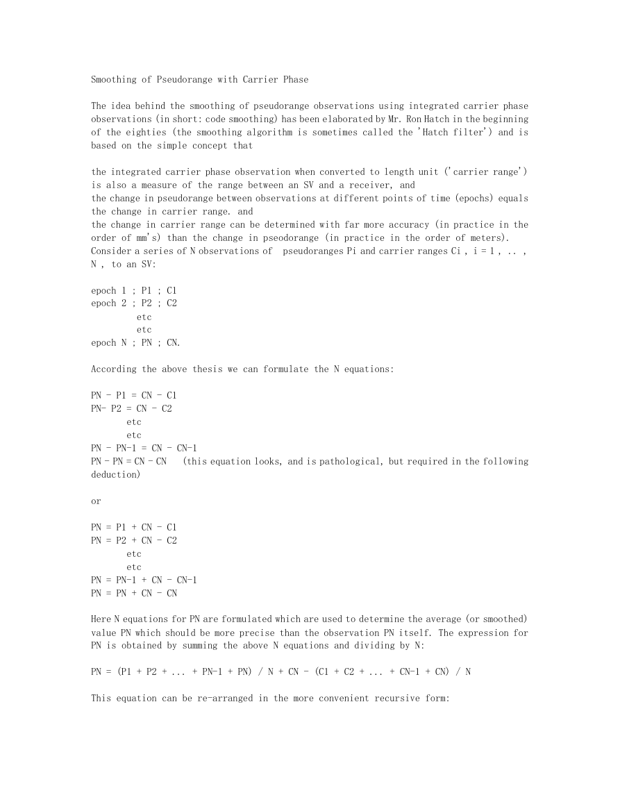According the above thesis we can formulate the N equations: PN - P1 = CN - C1 PN- P2 = CN - C2 etc etc PN - PN-1 = CN - CN-1 PN - PN = CN - CN deduction) (this equation looks, and is pathological, but required in the following or PN = P1 + CN - C1 PN = P2 + CN - C2 etc etc PN = PN-1 + CN - CN-1 PN = PN + CN - CN Here N equations for PN are formulated which are used to determine the average (or smoothed) value PN which should be more precise than the observation PN itself. The expression for PN is obtained by summing the above N equations and dividing by N: PN = (P1 + P2 + ... + PN-1 + PN) / N + CN - (C1 + C2 + ... + CN-1 + CN) / N This equation can be re-arranged in the more convenient recursive form: 

PN = PN / N + (PN-1 + CN - CN-1) * (N - 1) / N with PN-1 the smoothed pseudorange of the previous epoch. The above re-arranging is straight forward and is left as an exercise to the reader (that's what my textbooks used to say about insolvable problems, and I like to get some revenge at this moment !) In principle the more epochs of data are used in the smoothing process the more precise the smoothed pseudorange should become, and should approach the precision of the carrier range (remember: mm-level). In practise there are always facts which destroy the ideal world. Since the ionosphere delays the pseudorange and advances the carrier range (see the theory page) the change in pseudorange does not equal exactly the change in carrier range (this effect is called the ionospheric divergence). If the receiver channel looses lock on the SV momentarily, or if the range rate of change is too high, the carrier phase integration process is disrupted, resulting in a 'cycle slip', and an incorrect change in carrier range. To overcome the above drawbacks the number of observations used to smooth the pseudoranges is limited. At one observation per second a maximum of 100 seems a good value. Moreover, large cycle slips can be detected : if the carrier rate of change is larger by a certain margin than the pseudorange rate of change, a cycle slip is declared and the smoothing algorithm is reset (n = 1). The margin depends very much on the noise- and multipath figures of your receiver and the antenna location. For high quality receivers with optimally located antennas the margin could be as low as 1 m, a value of 15 m is more realistic, which implies that slips of more than 100 cycles (1 cycle is about 0.2 m) remain undetected. The limit value for N limits the error in the smoothed pseudorange, and lets it fade away after one to two minutes. Code smoothing reduces multipath and receiver noise on the pseudoranges. Although theoretically a reduction of a factor 10 can be reached, you can count on a reduction of at least a factor 2, and with some luck 5. Code smoothing does not improve the stand alone position very much, because the errors induced by Selective Availbility are far larger than the reduction in pseodorange noise and multipath. For differential code GPS the multipath and noise may very well be the largest contributions to the error budget, and in this case code smoothing does a good job. OK, enough with the dull theory, let's look at the implementation of the code smoothing concept with single difference processing.. I start with the remark, that at this point in the s/w pages it's the first time that we discuss time series of observations in stead of observations at one epoch only. Its for this reason, that I added some overhead s/w to process time series in stead of one epoch. And in order to conserve disk space (my provider limits me), and for clarity I removed all procedures and functions which were formulated in earlier examples. If you want to run the example code, you should copy the procedures and functions from the single difference example code. View/ download the example code by clicking here. I also prepared files with reference receiver data, , moving receiver data and support data, with observations of about 100 epochs of data taken from two stationary receivers, and the output , as generated by the program. 

The position noise in the ouput file is very low, I collected this data with very good receivers. Experiment with the data by changing the maximum value of the number of observations (Nmax in procedure 'readsmooth') to a lower value, or switch off the filter by setting Nmax to 1. Have fun !