Matrix Calculus:
Derivation and Simple Application
HU, Pili∗
March 30, 2012†
Abstract
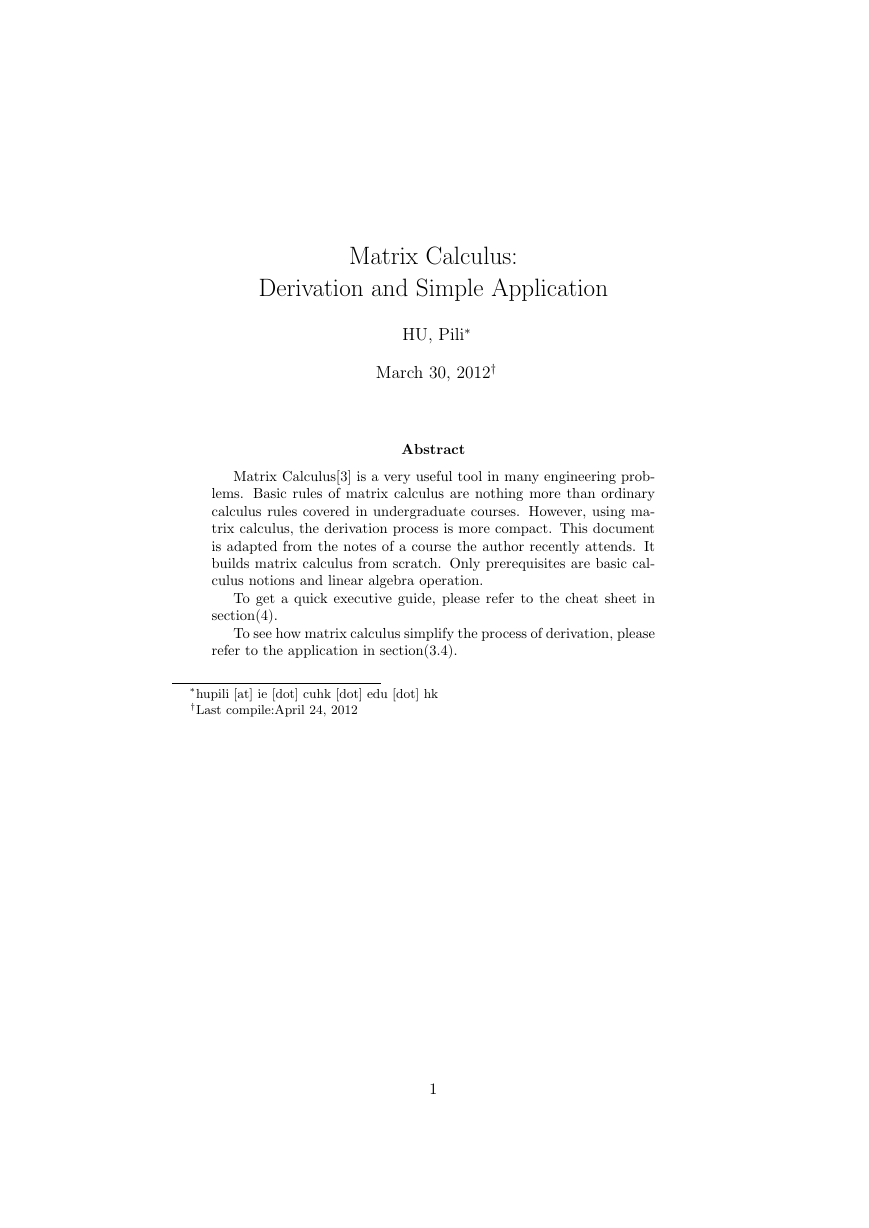
Matrix Calculus[3] is a very useful tool in many engineering prob-
lems. Basic rules of matrix calculus are nothing more than ordinary
calculus rules covered in undergraduate courses. However, using ma-
trix calculus, the derivation process is more compact. This document
is adapted from the notes of a course the author recently attends. It
builds matrix calculus from scratch. Only prerequisites are basic cal-
culus notions and linear algebra operation.
To get a quick executive guide, please refer to the cheat sheet in
section(4).
To see how matrix calculus simplify the process of derivation, please
refer to the application in section(3.4).
∗hupili [at] ie [dot] cuhk [dot] edu [dot] hk
†Last compile:April 24, 2012
1
�
HU, Pili
Contents
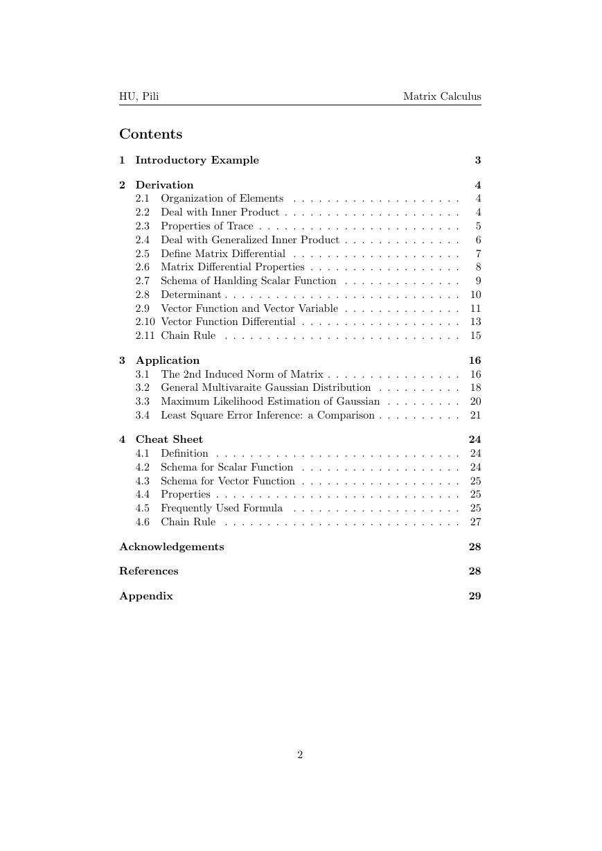
1 Introductory Example
2 Derivation
Matrix Calculus
3
4
4
4
5
6
7
8
9
10
11
13
15
16
16
18
20
21
24
24
24
25
25
25
27
28
28
29
2.1 Organization of Elements
. . . . . . . . . . . . . . . . . . . .
2.2 Deal with Inner Product . . . . . . . . . . . . . . . . . . . . .
2.3 Properties of Trace . . . . . . . . . . . . . . . . . . . . . . . .
2.4 Deal with Generalized Inner Product . . . . . . . . . . . . . .
2.5 Define Matrix Differential
. . . . . . . . . . . . . . . . . . . .
2.6 Matrix Differential Properties . . . . . . . . . . . . . . . . . .
2.7 Schema of Hanlding Scalar Function . . . . . . . . . . . . . .
2.8 Determinant . . . . . . . . . . . . . . . . . . . . . . . . . . . .
2.9 Vector Function and Vector Variable . . . . . . . . . . . . . .
2.10 Vector Function Differential
. . . . . . . . . . . . . . . . . . .
2.11 Chain Rule . . . . . . . . . . . . . . . . . . . . . . . . . . . .
3 Application
3.1 The 2nd Induced Norm of Matrix . . . . . . . . . . . . . . . .
3.2 General Multivaraite Gaussian Distribution . . . . . . . . . .
3.3 Maximum Likelihood Estimation of Gaussian . . . . . . . . .
3.4 Least Square Error Inference: a Comparison . . . . . . . . . .
4 Cheat Sheet
4.1 Definition . . . . . . . . . . . . . . . . . . . . . . . . . . . . .
4.2 Schema for Scalar Function . . . . . . . . . . . . . . . . . . .
4.3 Schema for Vector Function . . . . . . . . . . . . . . . . . . .
4.4 Properties . . . . . . . . . . . . . . . . . . . . . . . . . . . . .
4.5 Frequently Used Formula . . . . . . . . . . . . . . . . . . . .
4.6 Chain Rule . . . . . . . . . . . . . . . . . . . . . . . . . . . .
Acknowledgements
References
Appendix
2
�
HU, Pili
Matrix Calculus
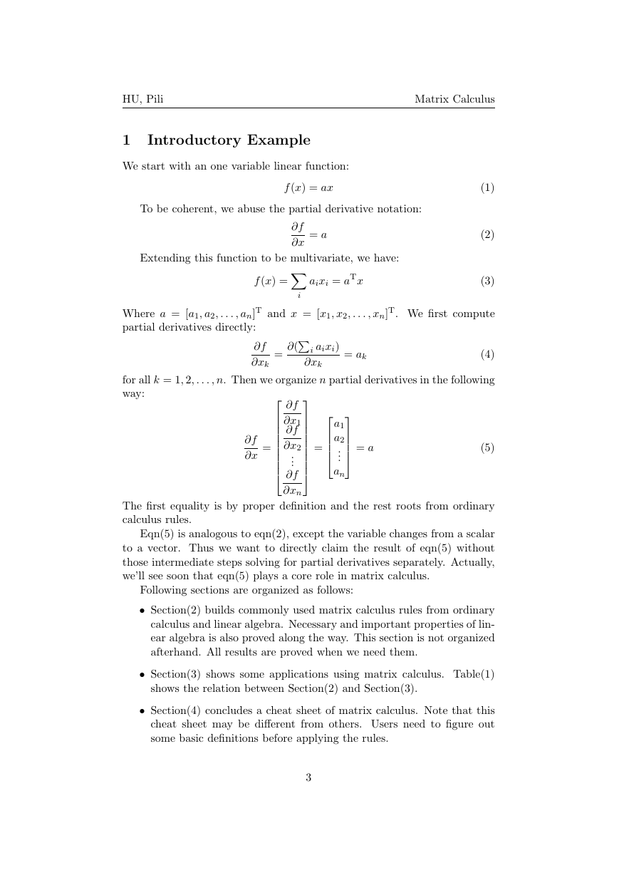
1
Introductory Example
We start with an one variable linear function:
f (x) = ax
To be coherent, we abuse the partial derivative notation:
(1)
(2)
(3)
(5)
Extending this function to be multivariate, we have:
f (x) =
aixi = aTx
Where a = [a1, a2, . . . , an]T and x = [x1, x2, . . . , xn]T. We first compute
partial derivatives directly:
∂f
∂xk
i aixi)
∂xk
= ak
(4)
for all k = 1, 2, . . . , n. Then we organize n partial derivatives in the following
way:
= a
∂f
∂x
i
∂(
=
∂f
∂x1
∂f
∂x2
...
∂f
∂xn
=
= a
a1
a2
...
an
∂f
∂x
=
The first equality is by proper definition and the rest roots from ordinary
calculus rules.
Eqn(5) is analogous to eqn(2), except the variable changes from a scalar
to a vector. Thus we want to directly claim the result of eqn(5) without
those intermediate steps solving for partial derivatives separately. Actually,
we’ll see soon that eqn(5) plays a core role in matrix calculus.
Following sections are organized as follows:
• Section(2) builds commonly used matrix calculus rules from ordinary
calculus and linear algebra. Necessary and important properties of lin-
ear algebra is also proved along the way. This section is not organized
afterhand. All results are proved when we need them.
• Section(3) shows some applications using matrix calculus. Table(1)
shows the relation between Section(2) and Section(3).
• Section(4) concludes a cheat sheet of matrix calculus. Note that this
cheat sheet may be different from others. Users need to figure out
some basic definitions before applying the rules.
3
�
HU, Pili
Matrix Calculus
Table 1: Derivation and Application Correspondance
Derivation Application
2.1-2.7
2.9,2.10
2.8,2.11
3.1
3.2
3.3
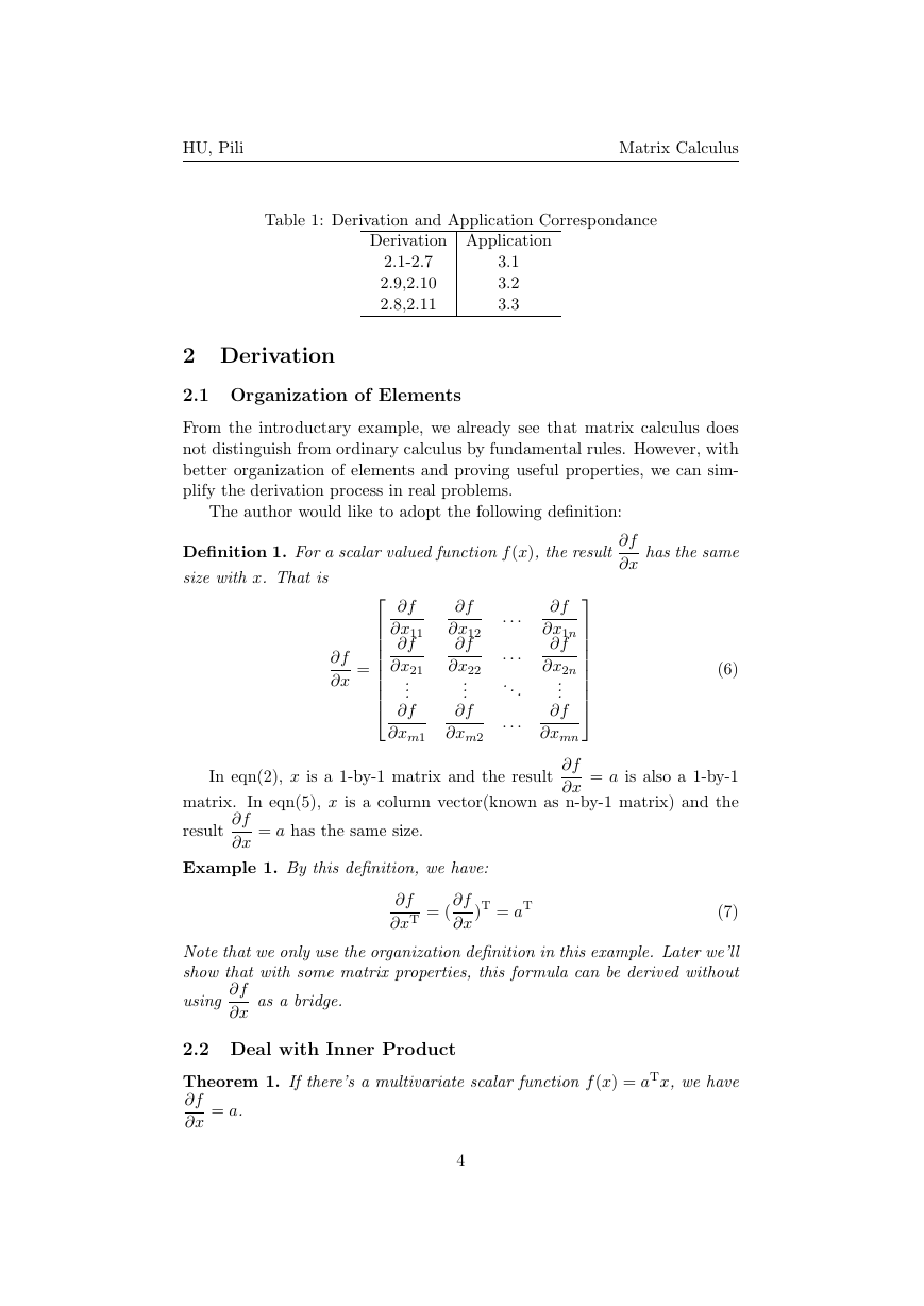
2 Derivation
2.1 Organization of Elements
From the introductary example, we already see that matrix calculus does
not distinguish from ordinary calculus by fundamental rules. However, with
better organization of elements and proving useful properties, we can sim-
plify the derivation process in real problems.
The author would like to adopt the following definition:
Definition 1. For a scalar valued function f (x), the result
size with x. That is
∂f
∂x
has the same
(6)
∂f
∂x
=
∂f
∂x11
∂f
∂x21
...
∂f
∂xm1
∂f
∂x12
∂f
∂x22
...
∂f
∂xm2
. . .
. . .
. . .
. . .
∂f
∂x1n
∂f
∂x2n
...
∂f
∂xmn
∂f
∂x
In eqn(2), x is a 1-by-1 matrix and the result
= a is also a 1-by-1
matrix. In eqn(5), x is a column vector(known as n-by-1 matrix) and the
result
∂f
∂x
= a has the same size.
Example 1. By this definition, we have:
∂f
∂xT = (
∂f
∂x
)T = aT
(7)
Note that we only use the organization definition in this example. Later we’ll
show that with some matrix properties, this formula can be derived without
using
as a bridge.
∂f
∂x
2.2 Deal with Inner Product
Theorem 1. If there’s a multivariate scalar function f (x) = aTx, we have
∂f
∂x
= a.
4
�
HU, Pili
Matrix Calculus
Proof. See introductary example.
Thus,
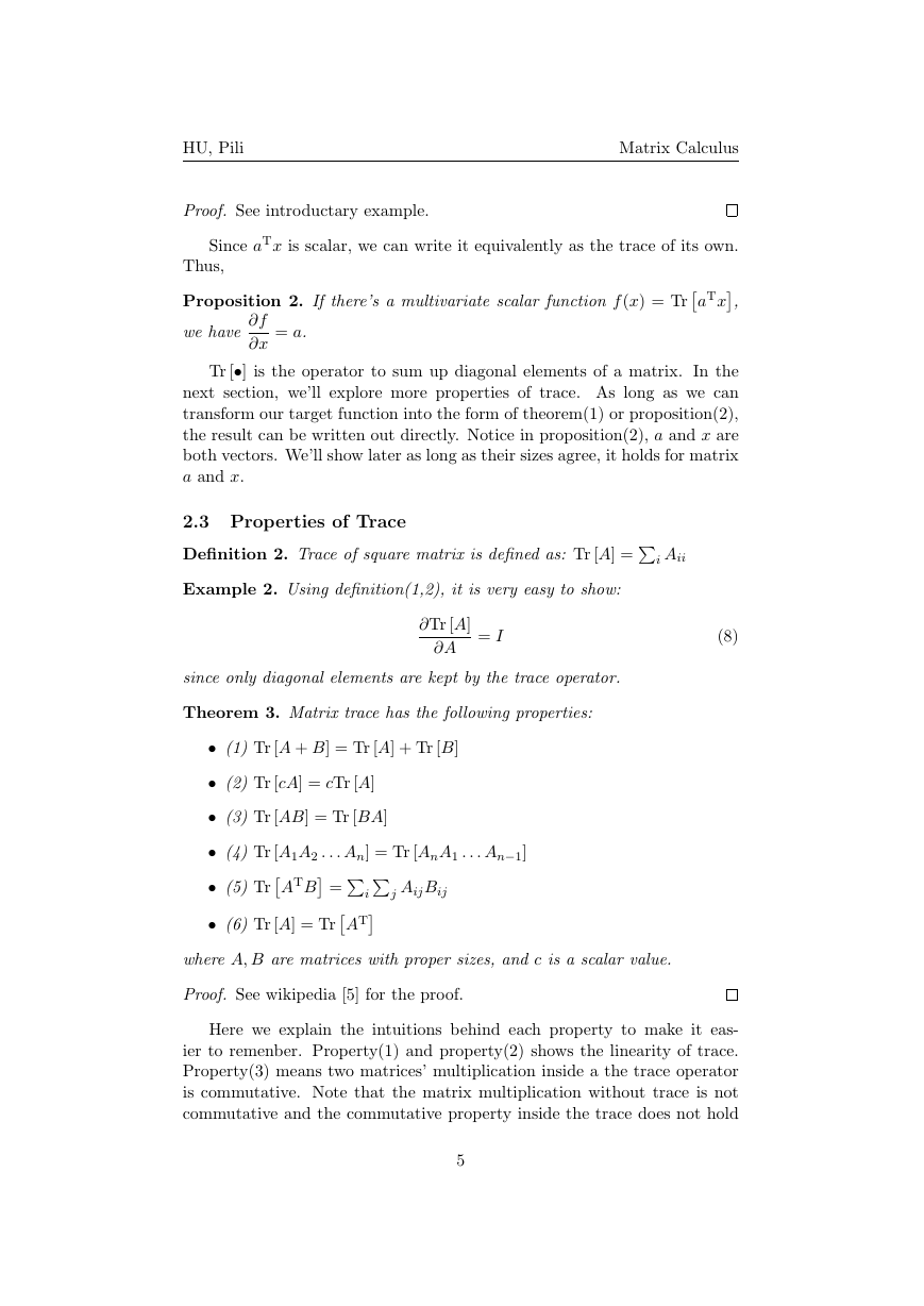
Since aTx is scalar, we can write it equivalently as the trace of its own.
Proposition 2. If there’s a multivariate scalar function f (x) = TraTx,
we have
= a.
∂f
∂x
Tr [•] is the operator to sum up diagonal elements of a matrix. In the
next section, we’ll explore more properties of trace. As long as we can
transform our target function into the form of theorem(1) or proposition(2),
the result can be written out directly. Notice in proposition(2), a and x are
both vectors. We’ll show later as long as their sizes agree, it holds for matrix
a and x.
2.3 Properties of Trace
Definition 2. Trace of square matrix is defined as: Tr [A] =
i Aii
Example 2. Using definition(1,2), it is very easy to show:
∂Tr [A]
∂A
= I
(8)
since only diagonal elements are kept by the trace operator.
Theorem 3. Matrix trace has the following properties:
• (1) Tr [A + B] = Tr [A] + Tr [B]
• (2) Tr [cA] = cTr [A]
• (3) Tr [AB] = Tr [BA]
• (4) Tr [A1A2 . . . An] = Tr [AnA1 . . . An−1]
• (5) TrATB =
• (6) Tr [A] = TrAT
i
j AijBij
where A, B are matrices with proper sizes, and c is a scalar value.
Proof. See wikipedia [5] for the proof.
Here we explain the intuitions behind each property to make it eas-
ier to remenber. Property(1) and property(2) shows the linearity of trace.
Property(3) means two matrices’ multiplication inside a the trace operator
is commutative. Note that the matrix multiplication without trace is not
commutative and the commutative property inside the trace does not hold
5
�
HU, Pili
Matrix Calculus
for more than 2 matrices. Property (4) is the proposition of property (3) by
considering A1A2 . . . An−1 as a whole. It is known as cyclic property, so that
you can rotate the matrices inside a trace operator. Property (5) shows a
way to express the sum of element by element product using matrix product
and trace. Note that inner product of two vectors is also the sum of ele-
ment by element product. Property (5) resembles the vector inner product
by form(ATB). The author regards property (5) as the extension of inner
product to matrices(Generalized Inner Product).
2.4 Deal with Generalized Inner Product
Theorem 4. If there’s a multivariate scalar function f (x) = TrATx, we
have
∂f
∂x
= A. (A, x can be matrices).
Proof. Using property (5) of trace, we can write f as:
f (x) = TrATx =
Aijxij
∂(
ij
ij Aijxij)
∂xij
= Aij
It’s easy to show:
∂f
∂xij
=
Organize elements using definition(1), it is proved.
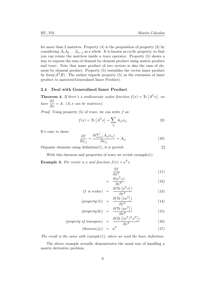
With this theorem and properties of trace we revisit example(1).
Example 3. For vector a, x and function f (x) = aTx
=
(f is scalar) =
(property(3)) =
(property(6)) =
(property of transpose) =
∂f
∂xT
∂(aTx)
∂xT
∂(TraTx)
∂(TrxaT)
∂(TraxT)
∂(Tr(aT)TxT)
∂xT
∂xT
∂xT
∂xT
(theorem(4)) = aT
(9)
(10)
(11)
(12)
(13)
(14)
(15)
(16)
(17)
The result is the same with example(1), where we used the basic definition.
The above example actually demonstrates the usual way of handling a
matrix derivative problem.
6
�
HU, Pili
Matrix Calculus
2.5 Define Matrix Differential
Although we want matrix derivative at most time, it turns out matrix differ-
ential is easier to operate due to the form invariance property of differential.
Matrix differential inherit this property as a natural consequence of the fol-
lowing definition.
Definition 3. Define matrix differential:
dA11
dA21
...
dA12
dA22
...
dAm1 dAm2
. . . dA1n
. . . dA2n
. . .
. . . dAmn
...
(18)
dA =
Theorem 5. Differential operator is distributive through trace operator:
dTr [A] = Tr [dA]
Proof.
LHS = d(
Aii) =
i
dA11
dA21
...
i
i
dAii
dA12
dA22
...
. . . dA1n
. . . dA2n
. . .
. . . dAmn
...
(19)
(20)
(21)
RHS = Tr
dAm1 dAm2
=
dAii = LHS
Now that matrix differential is well defined, we want to relate it back
to matrix derivative. The scalar version differential and derivative can be
related as follows:
df =
dx
(22)
∂f
∂x
So far, we’re dealing with scalar function f and matrix variable x.
and
dx are both matrix according to definition. In order to make the quantities
in eqn(22) equal, we must figure out a way to make the RHS a scalar. It’s
not surprising that trace is what we want.
∂f
∂x
Theorem 6.
df = Tr
(
∂f
∂x
)Tdx
for scalar function f and arbitrarily sized x.
7
(23)
�
HU, Pili
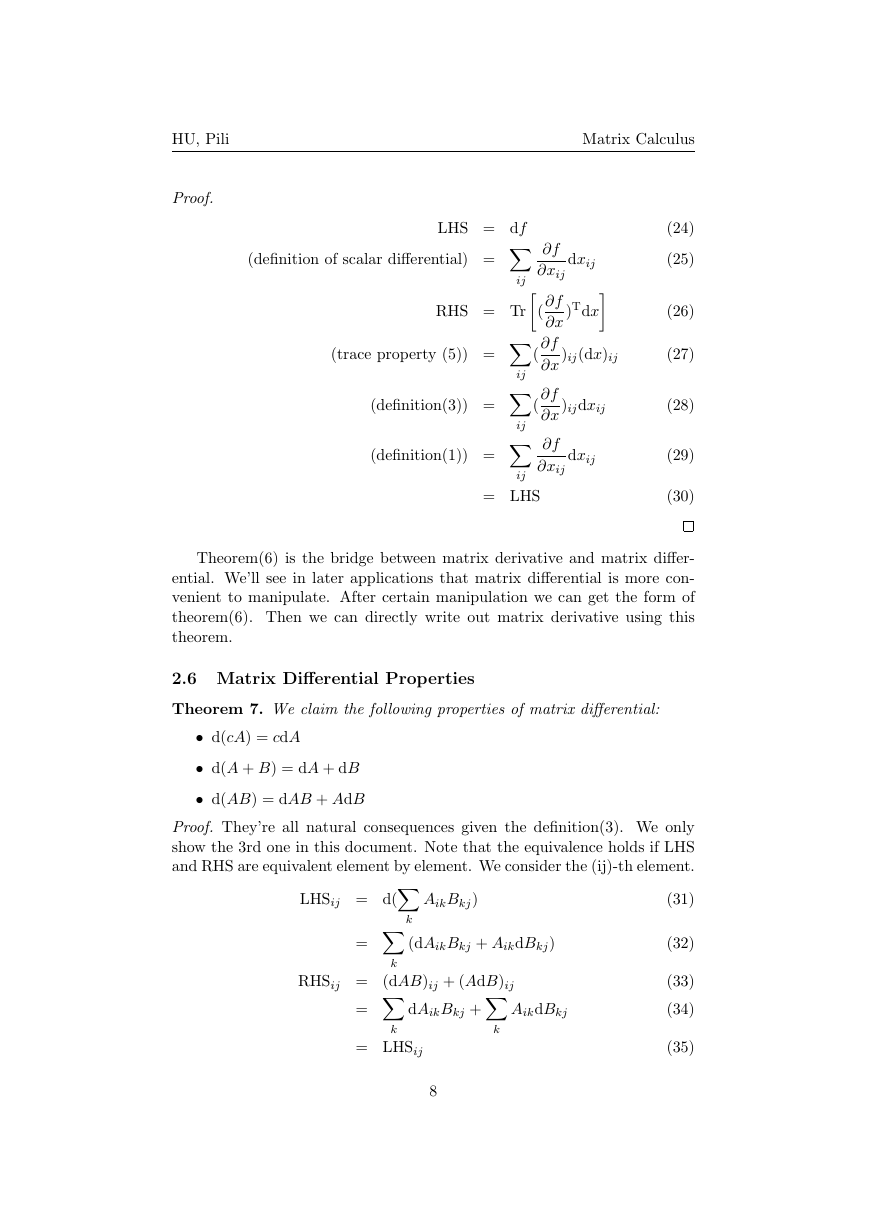
Proof.
(definition of scalar differential) =
LHS = df
Matrix Calculus
RHS = Tr
(
)Tdx
ij
ij
ij
(
ij
∂f
∂xij
dxij
∂f
∂x
∂f
∂x
)ij(dx)ij
(
∂f
∂x
)ijdxij
∂f
∂xij
dxij
= LHS
(trace property (5)) =
(definition(3)) =
(definition(1)) =
(24)
(25)
(26)
(27)
(28)
(29)
(30)
(31)
(32)
(33)
(34)
(35)
Theorem(6) is the bridge between matrix derivative and matrix differ-
ential. We’ll see in later applications that matrix differential is more con-
venient to manipulate. After certain manipulation we can get the form of
theorem(6). Then we can directly write out matrix derivative using this
theorem.
2.6 Matrix Differential Properties
Theorem 7. We claim the following properties of matrix differential:
• d(cA) = cdA
• d(A + B) = dA + dB
• d(AB) = dAB + AdB
Proof. They’re all natural consequences given the definition(3). We only
show the 3rd one in this document. Note that the equivalence holds if LHS
and RHS are equivalent element by element. We consider the (ij)-th element.
k
k
=
=
LHSij = d(
AikBkj)
(dAikBkj + AikdBkj)
RHSij = (dAB)ij + (AdB)ij
dAikBkj +
AikdBkj
k
= LHSij
k
8
�



 2023年江西萍乡中考道德与法治真题及答案.doc
 2012年重庆南川中考生物真题及答案.doc
 2013年江西师范大学地理学综合及文艺理论基础考研真题.doc
 2020年四川甘孜小升初语文真题及答案I卷.doc
 2020年注册岩土工程师专业基础考试真题及答案.doc
 2023-2024学年福建省厦门市九年级上学期数学月考试题及答案.doc
 2021-2022学年辽宁省沈阳市大东区九年级上学期语文期末试题及答案.doc
 2022-2023学年北京东城区初三第一学期物理期末试卷及答案.doc
 2018上半年江西教师资格初中地理学科知识与教学能力真题及答案.doc
 2012年河北国家公务员申论考试真题及答案-省级.doc
 2020-2021学年江苏省扬州市江都区邵樊片九年级上学期数学第一次质量检测试题及答案.doc
 2022下半年黑龙江教师资格证中学综合素质真题及答案.doc