Realtime Multi-Person 2D Pose Estimation using Part Affinity Fields ∗
Zhe Cao
Tomas Simon
Shih-En Wei
Yaser Sheikh
The Robotics Institute, Carnegie Mellon University
{zhecao,shihenw}@cmu.edu
{tsimon,yaser}@cs.cmu.edu
Abstract
We present an approach to efficiently detect the 2D pose
of multiple people in an image. The approach uses a non-
parametric representation, which we refer to as Part Affinity
Fields (PAFs), to learn to associate body parts with individ-
uals in the image. The architecture encodes global con-
text, allowing a greedy bottom-up parsing step that main-
tains high accuracy while achieving realtime performance,
irrespective of the number of people in the image. The ar-
chitecture is designed to jointly learn part locations and
their association via two branches of the same sequential
prediction process. Our method placed first in the inaugu-
ral COCO 2016 keypoints challenge, and significantly ex-
ceeds the previous state-of-the-art result on the MPII Multi-
Person benchmark, both in performance and efficiency.
1. Introduction
Human 2D pose estimation—the problem of localizing
anatomical keypoints or “parts”—has largely focused on
finding body parts of individuals [8, 4, 3, 21, 33, 13, 25, 31,
6, 24]. Inferring the pose of multiple people in images, es-
pecially socially engaged individuals, presents a unique set
of challenges. First, each image may contain an unknown
number of people that can occur at any position or scale.
Second, interactions between people induce complex spa-
tial interference, due to contact, occlusion, and limb articu-
lations, making association of parts difficult. Third, runtime
complexity tends to grow with the number of people in the
image, making realtime performance a challenge.
A common approach [23, 9, 27, 12, 19] is to employ
a person detector and perform single-person pose estima-
tion for each detection. These top-down approaches di-
rectly leverage existing techniques for single-person pose
estimation [17, 31, 18, 28, 29, 7, 30, 5, 6, 20], but suffer
from early commitment: if the person detector fails–as it
is prone to do when people are in close proximity–there is
no recourse to recovery. Furthermore, the runtime of these
∗Video result: https://youtu.be/pW6nZXeWlGM
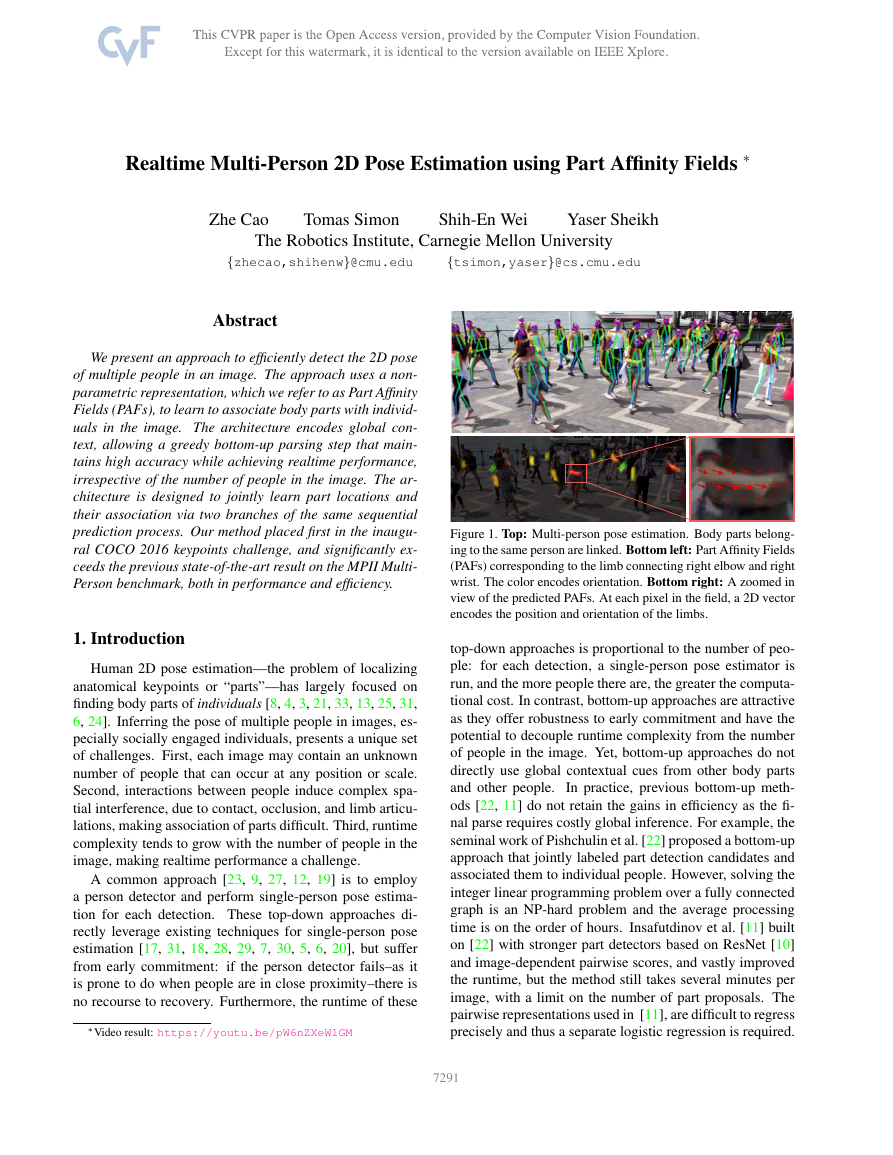
Figure 1. Top: Multi-person pose estimation. Body parts belong-
ing to the same person are linked. Bottom left: Part Affinity Fields
(PAFs) corresponding to the limb connecting right elbow and right
wrist. The color encodes orientation. Bottom right: A zoomed in
view of the predicted PAFs. At each pixel in the field, a 2D vector
encodes the position and orientation of the limbs.
top-down approaches is proportional to the number of peo-
ple: for each detection, a single-person pose estimator is
run, and the more people there are, the greater the computa-
tional cost. In contrast, bottom-up approaches are attractive
as they offer robustness to early commitment and have the
potential to decouple runtime complexity from the number
of people in the image. Yet, bottom-up approaches do not
directly use global contextual cues from other body parts
and other people.
In practice, previous bottom-up meth-
ods [22, 11] do not retain the gains in efficiency as the fi-
nal parse requires costly global inference. For example, the
seminal work of Pishchulin et al. [22] proposed a bottom-up
approach that jointly labeled part detection candidates and
associated them to individual people. However, solving the
integer linear programming problem over a fully connected
graph is an NP-hard problem and the average processing
time is on the order of hours. Insafutdinov et al. [11] built
on [22] with stronger part detectors based on ResNet [10]
and image-dependent pairwise scores, and vastly improved
the runtime, but the method still takes several minutes per
image, with a limit on the number of part proposals. The
pairwise representations used in [11], are difficult to regress
precisely and thus a separate logistic regression is required.
17291
�
(b) Part Confidence Maps
(a) Input Image
(c) Part Affinity Fields
(d) Bipartite Matching
(e) Parsing Results
Figure 2. Overall pipeline. Our method takes the entire image as the input for a two-branch CNN to jointly predict confidence maps for
body part detection, shown in (b), and part affinity fields for parts association, shown in (c). The parsing step performs a set of bipartite
matchings to associate body parts candidates (d). We finally assemble them into full body poses for all people in the image (e).
In this paper, we present an efficient method for multi-
person pose estimation with state-of-the-art accuracy on
multiple public benchmarks. We present the first bottom-up
representation of association scores via Part Affinity Fields
(PAFs), a set of 2D vector fields that encode the location
and orientation of limbs over the image domain. We demon-
strate that simultaneously inferring these bottom-up repre-
sentations of detection and association encode global con-
text sufficiently well to allow a greedy parse to achieve
high-quality results, at a fraction of the computational cost.
We have publically released the code for full reproducibil-
ity, presenting the first realtime system for multi-person 2D
pose detection.
3
t
2. Method
Fig. 2 illustrates the overall pipeline of our method. The
system takes, as input, a color image of size w × h (Fig. 2a)
and produces, as output, the 2D locations of anatomical key-
points for each person in the image (Fig. 2e). First, a feed-
forward network simultaneously predicts a set of 2D con-
fidence maps S of body part locations (Fig. 2b) and a set
of 2D vector fields L of part affinities, which encode the
degree of association between parts (Fig. 2c). The set S =
(S1, S2, ..., SJ ) has J confidence maps, one per part, where
Sj ∈ Rw×h, j ∈ {1 . . . J}. The set L = (L1, L2, ..., LC)
has C vector fields, one per limb1, where Lc ∈ Rw×h×2,
c ∈ {1 . . . C}, each image location in Lc encodes a 2D vec-
tor (as shown in Fig. 1). Finally, the confidence maps and
the affinity fields are parsed by greedy inference (Fig. 2d)
to output the 2D keypoints for all people in the image.
2.1. Simultaneous Detection and Association
Our architecture, shown in Fig. 3, simultaneously pre-
dicts detection confidence maps and affinity fields that en-
code part-to-part association. The network is split into two
branches: the top branch, shown in beige, predicts the con-
fidence maps, and the bottom branch, shown in blue, pre-
dicts the affinity fields. Each branch is an iterative predic-
1We refer to part pairs as limbs for clarity, despite the fact that some
pairs are not human limbs (e.g., the face).
Stage 1
Stage t, (t ≥ 2)
C
Branch 1
ρ1
Convolution
3×3
3×3
C
C
3×3
3×3
C
C
3×3
3×3
C
C
1×1
1×1
C
C
1×1
1×1
C
C
F
3×3
C
3×3
C
3×3
C
1×1
C
1×1
C
Branch 2
φ1
Loss
f 1
1
S1
h0×w0
h0×w0
L1
Loss
f 1
2
Branch 1
ρt
Loss
f t
1
7×7
C
7×7
C
7×7
C
7×7
C
7×7
C
1×1
C
1×1
C
h0×w0
St
7×7
C
7×7
C
7×7
C
7×7
C
7×7
C
1×1
C
1×1
C
Branch 2
φt
h0×w0
Lt
Loss
f t
2
Figure 3. Architecture of the two-branch multi-stage CNN. Each
stage in the first branch predicts confidence maps St, and each
stage in the second branch predicts PAFs Lt. After each stage, the
predictions from the two branches, along with the image features,
are concatenated for next stage.
tion architecture, following Wei et al. [31], which refines
the predictions over successive stages, t ∈ {1, . . . , T }, with
intermediate supervision at each stage.
The image is first analyzed by a convolutional network
(initialized by the first 10 layers of VGG-19 [26] and fine-
tuned), generating a set of feature maps F that is input to
the first stage of each branch. At the first stage, the network
produces a set of detection confidence maps S1 = ρ1(F)
and a set of part affinity fields L1 = φ1(F), where ρ1 and
φ1 are the CNNs for inference at Stage 1. In each subse-
quent stage, the predictions from both branches in the pre-
vious stage, along with the original image features F, are
concatenated and used to produce refined predictions,
St = ρt(F, St−1, Lt−1), ∀t ≥ 2,
Lt = φt(F, St−1, Lt−1), ∀t ≥ 2,
(1)
(2)
where ρt and φt are the CNNs for inference at Stage t.
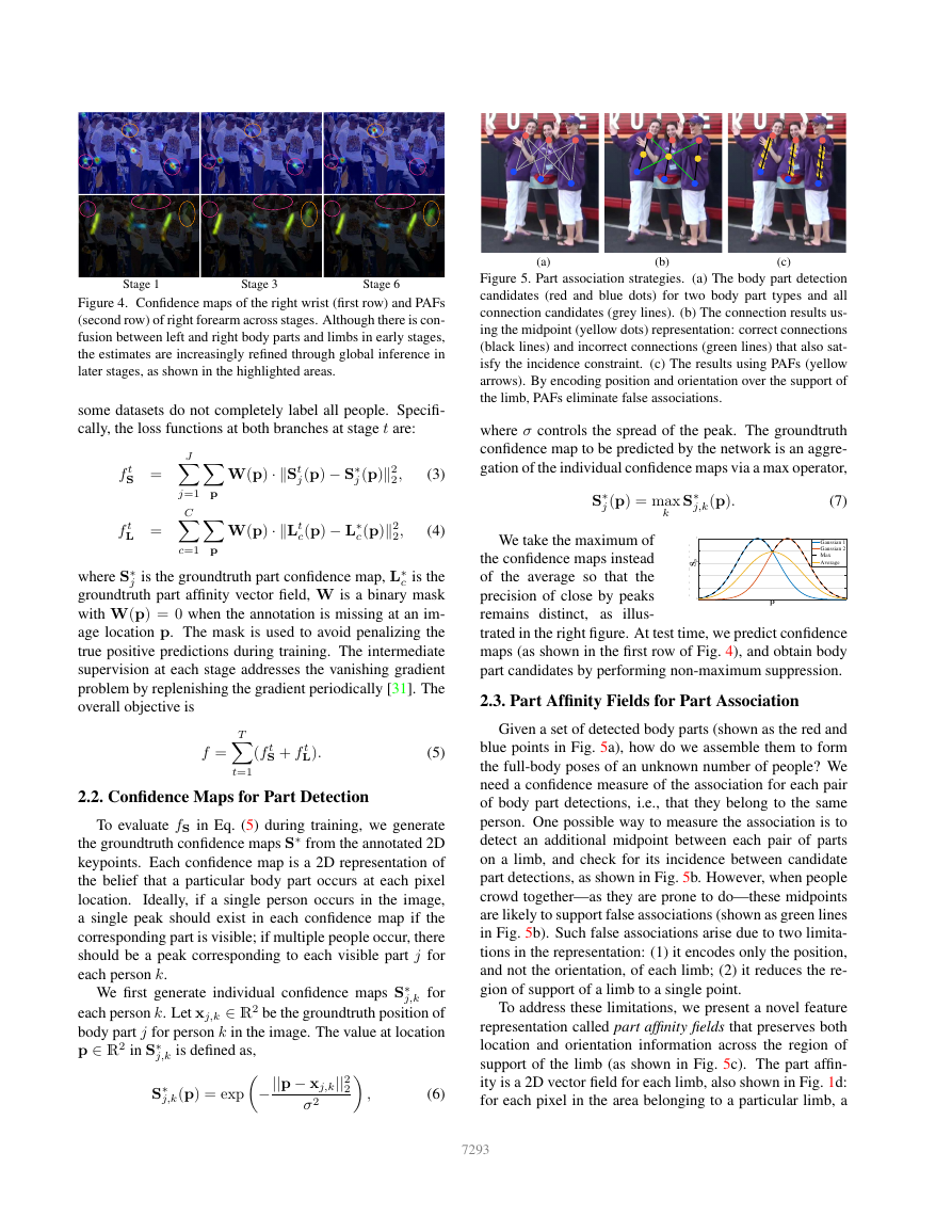
Fig. 4 shows the refinement of the confidence maps and
affinity fields across stages. To guide the network to iter-
atively predict confidence maps of body parts in the first
branch and PAFs in the second branch, we apply two loss
functions at the end of each stage, one at each branch re-
spectively. We use an L2 loss between the estimated predic-
tions and the groundtruth maps and fields. Here, we weight
the loss functions spatially to address a practical issue that
7292
�
Stage 1
Stage 3
Stage 6
Figure 4. Confidence maps of the right wrist (first row) and PAFs
(second row) of right forearm across stages. Although there is con-
fusion between left and right body parts and limbs in early stages,
the estimates are increasingly refined through global inference in
later stages, as shown in the highlighted areas.
some datasets do not completely label all people. Specifi-
cally, the loss functions at both branches at stage t are:
f t
S =
f t
L =
J
C
Xj=1Xp
Xc=1Xp
W(p) · kSt
j(p) − S∗
j (p)k2
2,
W(p) · kLt
c(p) − L∗
c (p)k2
2,
(3)
(4)
j is the groundtruth part confidence map, L∗
where S∗
c is the
groundtruth part affinity vector field, W is a binary mask
with W(p) = 0 when the annotation is missing at an im-
age location p. The mask is used to avoid penalizing the
true positive predictions during training. The intermediate
supervision at each stage addresses the vanishing gradient
problem by replenishing the gradient periodically [31]. The
overall objective is
f =
T
Xt=1
(f t
S + f t
L).
(5)
2.2. Confidence Maps for Part Detection
To evaluate fS in Eq. (5) during training, we generate
the groundtruth confidence maps S∗ from the annotated 2D
keypoints. Each confidence map is a 2D representation of
the belief that a particular body part occurs at each pixel
location.
Ideally, if a single person occurs in the image,
a single peak should exist in each confidence map if the
corresponding part is visible; if multiple people occur, there
should be a peak corresponding to each visible part j for
each person k.
We first generate individual confidence maps S∗
j,k for
each person k. Let xj,k ∈ R2 be the groundtruth position of
body part j for person k in the image. The value at location
p ∈ R2 in S∗
j,k is defined as,
S∗
j,k(p) = exp−
||p − xj,k||2
2
σ2
,
(6)
ns
ns
(a)
(b)
(c)
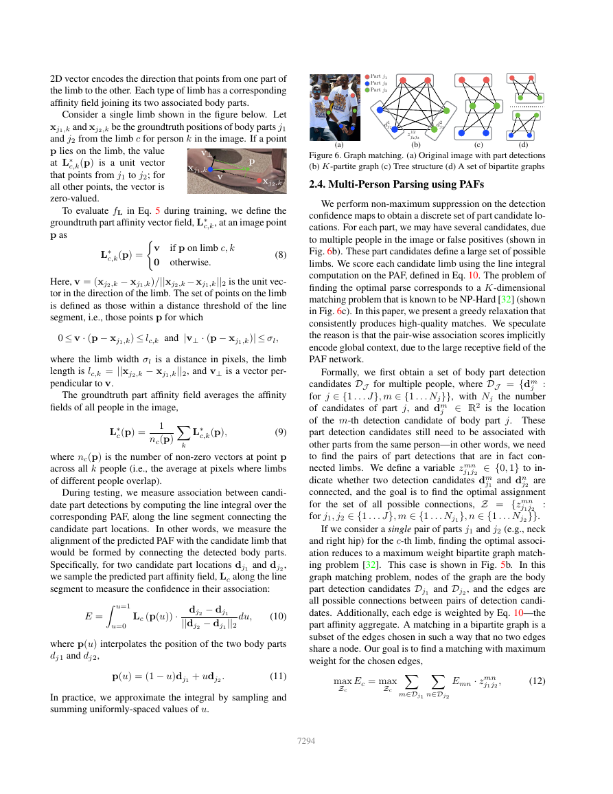
Figure 5. Part association strategies. (a) The body part detection
candidates (red and blue dots) for two body part types and all
connection candidates (grey lines). (b) The connection results us-
ing the midpoint (yellow dots) representation: correct connections
(black lines) and incorrect connections (green lines) that also sat-
isfy the incidence constraint. (c) The results using PAFs (yellow
arrows). By encoding position and orientation over the support of
the limb, PAFs eliminate false associations.
where σ controls the spread of the peak. The groundtruth
confidence map to be predicted by the network is an aggre-
gation of the individual confidence maps via a max operator,
S∗
j (p) = max
k
S∗
j,k(p).
(7)
0.9
0.7
0.6
0.8
0.8
1
1
p
0.6
S
S
0.5
We take the maximum of
the confidence maps instead
of the average so that the
precision of close by peaks
remains distinct, as illus-
trated in the right figure. At test time, we predict confidence
maps (as shown in the first row of Fig. 4), and obtain body
part candidates by performing non-maximum suppression.
Gaussian 1
Gaussian 1
Gaussian 2
Gaussian 2
Max
Max
Average
Average
p
p
0.1
0.4
0.3
0.2
0
0
0.4
0.2
2.3. Part Affinity Fields for Part Association
Given a set of detected body parts (shown as the red and
blue points in Fig. 5a), how do we assemble them to form
the full-body poses of an unknown number of people? We
need a confidence measure of the association for each pair
of body part detections, i.e., that they belong to the same
person. One possible way to measure the association is to
detect an additional midpoint between each pair of parts
on a limb, and check for its incidence between candidate
part detections, as shown in Fig. 5b. However, when people
crowd together—as they are prone to do—these midpoints
are likely to support false associations (shown as green lines
in Fig. 5b). Such false associations arise due to two limita-
tions in the representation: (1) it encodes only the position,
and not the orientation, of each limb; (2) it reduces the re-
gion of support of a limb to a single point.
To address these limitations, we present a novel feature
representation called part affinity fields that preserves both
location and orientation information across the region of
support of the limb (as shown in Fig. 5c). The part affin-
ity is a 2D vector field for each limb, also shown in Fig. 1d:
for each pixel in the area belonging to a particular limb, a
7293
�
2D vector encodes the direction that points from one part of
the limb to the other. Each type of limb has a corresponding
affinity field joining its two associated body parts.
Part j1
Part j2
Part j3
Consider a single limb shown in the figure below. Let
xj1,k and xj2,k be the groundtruth positions of body parts j1
and j2 from the limb c for person k in the image. If a point
p lies on the limb, the value
at L∗
c,k(p) is a unit vector
that points from j1 to j2; for
all other points, the vector is
zero-valued.
xj1,k
xj2,k
p
v⊥
v
p
p
To evaluate fL in Eq. 5 during training, we define the
c,k, at an image point
groundtruth part affinity vector field, L∗
p as
L∗
c,k(p) =(v if p on limb c, k
0 otherwise.
(8)
Here, v = (xj2,k − xj1,k)/||xj2,k − xj1,k||2 is the unit vec-
tor in the direction of the limb. The set of points on the limb
is defined as those within a distance threshold of the line
segment, i.e., those points p for which
0 ≤ v · (p − xj1,k) ≤ lc,k and |v⊥ · (p − xj1,k)| ≤ σl,
where the limb width σl is a distance in pixels, the limb
length is lc,k = ||xj2,k − xj1,k||2, and v⊥ is a vector per-
pendicular to v.
The groundtruth part affinity field averages the affinity
fields of all people in the image,
L∗
c (p) =
L∗
c,k(p),
(9)
1
nc(p)Xk
where nc(p) is the number of non-zero vectors at point p
across all k people (i.e., the average at pixels where limbs
of different people overlap).
During testing, we measure association between candi-
date part detections by computing the line integral over the
corresponding PAF, along the line segment connecting the
candidate part locations. In other words, we measure the
alignment of the predicted PAF with the candidate limb that
would be formed by connecting the detected body parts.
Specifically, for two candidate part locations dj1 and dj2 ,
we sample the predicted part affinity field, Lc along the line
segment to measure the confidence in their association:
E =Z u=1
u=0
Lc (p(u)) ·
dj2 − dj1
||dj2 − dj1 ||2
du,
(10)
where p(u) interpolates the position of the two body parts
dj 1 and dj 2,
p(u) = (1 − u)dj1 + udj2 .
(11)
In practice, we approximate the integral by sampling and
summing uniformly-spaced values of u.
d1
j2
d2
j3
z12
j2j3
(b)
(a)
(c)
(d)
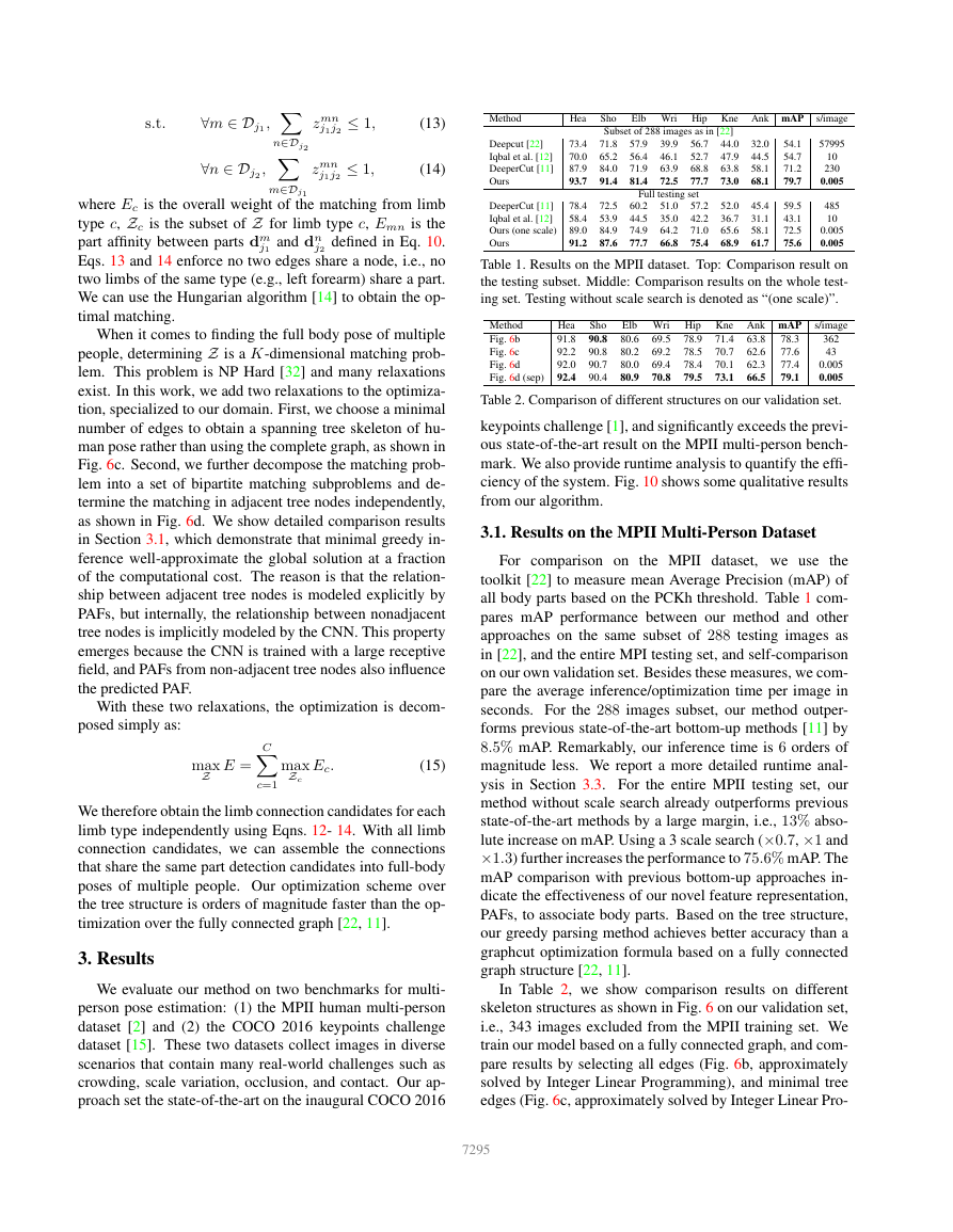
Figure 6. Graph matching. (a) Original image with part detections
(b) K-partite graph (c) Tree structure (d) A set of bipartite graphs
2.4. MultiPerson Parsing using PAFs
We perform non-maximum suppression on the detection
confidence maps to obtain a discrete set of part candidate lo-
cations. For each part, we may have several candidates, due
to multiple people in the image or false positives (shown in
Fig. 6b). These part candidates define a large set of possible
limbs. We score each candidate limb using the line integral
computation on the PAF, defined in Eq. 10. The problem of
finding the optimal parse corresponds to a K-dimensional
matching problem that is known to be NP-Hard [32] (shown
in Fig. 6c). In this paper, we present a greedy relaxation that
consistently produces high-quality matches. We speculate
the reason is that the pair-wise association scores implicitly
encode global context, due to the large receptive field of the
PAF network.
Formally, we first obtain a set of body part detection
candidates DJ for multiple people, where DJ = {dm
:
j
for j ∈ {1 . . . J}, m ∈ {1 . . . Nj}}, with Nj the number
of candidates of part j, and dm
j ∈ R2 is the location
of the m-th detection candidate of body part j. These
part detection candidates still need to be associated with
other parts from the same person—in other words, we need
to find the pairs of part detections that are in fact con-
nected limbs. We define a variable zmn
j1j2 ∈ {0, 1} to in-
dicate whether two detection candidates dm
j2 are
connected, and the goal is to find the optimal assignment
for the set of all possible connections, Z = {zmn
:
j1j2
for j1, j2 ∈ {1 . . . J}, m ∈ {1 . . . Nj1 }, n ∈ {1 . . . Nj2 }}.
j1 and dn
If we consider a single pair of parts j1 and j2 (e.g., neck
and right hip) for the c-th limb, finding the optimal associ-
ation reduces to a maximum weight bipartite graph match-
ing problem [32]. This case is shown in Fig. 5b. In this
graph matching problem, nodes of the graph are the body
part detection candidates Dj1 and Dj2 , and the edges are
all possible connections between pairs of detection candi-
dates. Additionally, each edge is weighted by Eq. 10—the
part affinity aggregate. A matching in a bipartite graph is a
subset of the edges chosen in such a way that no two edges
share a node. Our goal is to find a matching with maximum
weight for the chosen edges,
max
Zc
Ec = max
Zc Xm∈Dj1 Xn∈Dj2
Emn · zmn
j1j2 ,
(12)
7294
�
s.t.
∀m ∈ Dj1 , Xn∈Dj2
∀n ∈ Dj2 , Xm∈Dj1
zmn
j1j2 ≤ 1,
zmn
j1j2 ≤ 1,
(13)
(14)
where Ec is the overall weight of the matching from limb
type c, Zc is the subset of Z for limb type c, Emn is the
part affinity between parts dm
j2 defined in Eq. 10.
Eqs. 13 and 14 enforce no two edges share a node, i.e., no
two limbs of the same type (e.g., left forearm) share a part.
We can use the Hungarian algorithm [14] to obtain the op-
timal matching.
j1 and dn
When it comes to finding the full body pose of multiple
people, determining Z is a K-dimensional matching prob-
lem. This problem is NP Hard [32] and many relaxations
exist. In this work, we add two relaxations to the optimiza-
tion, specialized to our domain. First, we choose a minimal
number of edges to obtain a spanning tree skeleton of hu-
man pose rather than using the complete graph, as shown in
Fig. 6c. Second, we further decompose the matching prob-
lem into a set of bipartite matching subproblems and de-
termine the matching in adjacent tree nodes independently,
as shown in Fig. 6d. We show detailed comparison results
in Section 3.1, which demonstrate that minimal greedy in-
ference well-approximate the global solution at a fraction
of the computational cost. The reason is that the relation-
ship between adjacent tree nodes is modeled explicitly by
PAFs, but internally, the relationship between nonadjacent
tree nodes is implicitly modeled by the CNN. This property
emerges because the CNN is trained with a large receptive
field, and PAFs from non-adjacent tree nodes also influence
the predicted PAF.
With these two relaxations, the optimization is decom-
posed simply as:
max
Z
E =
C
Xc=1
max
Zc
Ec.
(15)
We therefore obtain the limb connection candidates for each
limb type independently using Eqns. 12- 14. With all limb
connection candidates, we can assemble the connections
that share the same part detection candidates into full-body
poses of multiple people. Our optimization scheme over
the tree structure is orders of magnitude faster than the op-
timization over the fully connected graph [22, 11].
3. Results
We evaluate our method on two benchmarks for multi-
person pose estimation: (1) the MPII human multi-person
dataset [2] and (2) the COCO 2016 keypoints challenge
dataset [15]. These two datasets collect images in diverse
scenarios that contain many real-world challenges such as
crowding, scale variation, occlusion, and contact. Our ap-
proach set the state-of-the-art on the inaugural COCO 2016
Elb Wri Hip Kne Ank mAP s/image
Method
Deepcut [22]
Iqbal et al. [12]
DeeperCut [11]
Ours
DeeperCut [11]
Iqbal et al. [12]
Ours (one scale)
Ours
Hea
73.4
70.0
87.9
93.7
78.4
58.4
89.0
91.2
Sho
Subset of 288 images as in [22]
71.8
65.2
84.0
91.4
57.9
56.4
71.9
81.4
56.7
52.7
68.8
77.7
39.9
46.1
63.9
72.5
44.0
47.9
63.8
73.0
Full testing set
72.5
53.9
84.9
87.6
60.2
44.5
74.9
77.7
51.0
35.0
64.2
66.8
57.2
42.2
71.0
75.4
52.0
36.7
65.6
68.9
32.0
44.5
58.1
68.1
45.4
31.1
58.1
61.7
54.1
54.7
71.2
79.7
59.5
43.1
72.5
75.6
57995
10
230
0.005
485
10
0.005
0.005
Table 1. Results on the MPII dataset. Top: Comparison result on
the testing subset. Middle: Comparison results on the whole test-
ing set. Testing without scale search is denoted as “(one scale)”.
Method
Fig. 6b
Fig. 6c
Fig. 6d
Fig. 6d (sep)
Hea
91.8
92.2
92.0
92.4
Sho
90.8
90.8
90.7
90.4
Elb Wri Hip Kne Ank mAP s/image
80.6
80.2
80.0
80.9
69.5
69.2
69.4
70.8
78.9
78.5
78.4
79.5
71.4
70.7
70.1
73.1
63.8
62.6
62.3
66.5
78.3
77.6
77.4
79.1
362
43
0.005
0.005
Table 2. Comparison of different structures on our validation set.
keypoints challenge [1], and significantly exceeds the previ-
ous state-of-the-art result on the MPII multi-person bench-
mark. We also provide runtime analysis to quantify the effi-
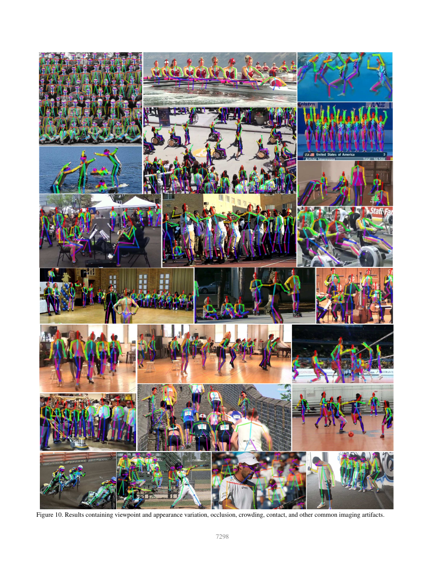
ciency of the system. Fig. 10 shows some qualitative results
from our algorithm.
3.1. Results on the MPII MultiPerson Dataset
For comparison on the MPII dataset, we use the
toolkit [22] to measure mean Average Precision (mAP) of
all body parts based on the PCKh threshold. Table 1 com-
pares mAP performance between our method and other
approaches on the same subset of 288 testing images as
in [22], and the entire MPI testing set, and self-comparison
on our own validation set. Besides these measures, we com-
pare the average inference/optimization time per image in
seconds. For the 288 images subset, our method outper-
forms previous state-of-the-art bottom-up methods [11] by
8.5% mAP. Remarkably, our inference time is 6 orders of
magnitude less. We report a more detailed runtime anal-
ysis in Section 3.3. For the entire MPII testing set, our
method without scale search already outperforms previous
state-of-the-art methods by a large margin, i.e., 13% abso-
lute increase on mAP. Using a 3 scale search (×0.7, ×1 and
×1.3) further increases the performance to 75.6% mAP. The
mAP comparison with previous bottom-up approaches in-
dicate the effectiveness of our novel feature representation,
PAFs, to associate body parts. Based on the tree structure,
our greedy parsing method achieves better accuracy than a
graphcut optimization formula based on a fully connected
graph structure [22, 11].
In Table 2, we show comparison results on different
skeleton structures as shown in Fig. 6 on our validation set,
i.e., 343 images excluded from the MPII training set. We
train our model based on a fully connected graph, and com-
pare results by selecting all edges (Fig. 6b, approximately
solved by Integer Linear Programming), and minimal tree
edges (Fig. 6c, approximately solved by Integer Linear Pro-
7295
�
%
n
o
i
s
i
c
e
r
p
e
g
a
r
e
v
a
n
a
e
M
100
90
80
70
60
50
40
30
20
10
0
%
n
o
i
s
i
c
e
r
p
e
g
a
r
e
v
a
n
a
e
M
100
90
80
70
60
50
40
30
20
10
0
GT detection
GT connection
PAFs with mask
PAFs
Two-midpoint
One-midpoint
1-stage
2-stage
3-stage
4-stage
5-stage
6-stage
0.1
0.2
0.3
0.4
0.5
0.1
0.2
0.3
0.4
0.5
Normalized distance
Normalized distance
(a)
(b)
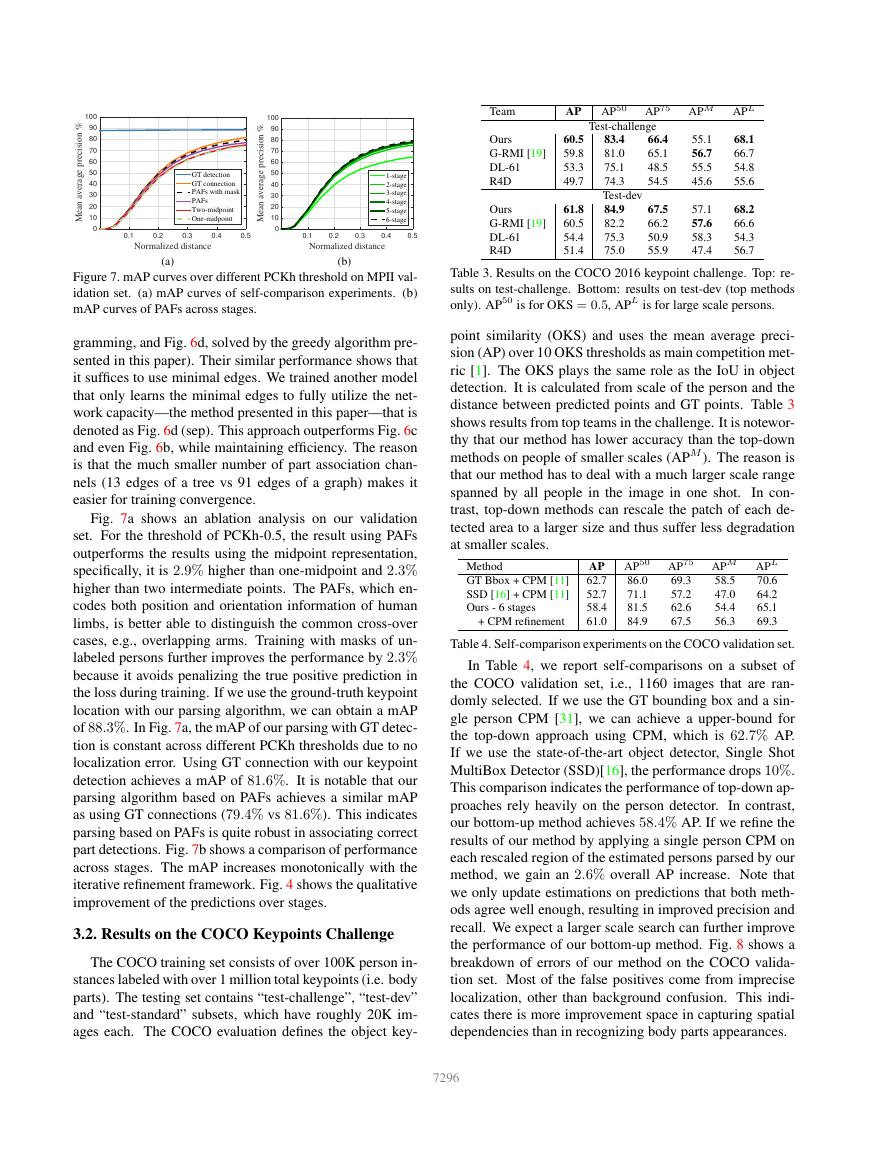
Figure 7. mAP curves over different PCKh threshold on MPII val-
idation set. (a) mAP curves of self-comparison experiments. (b)
mAP curves of PAFs across stages.
gramming, and Fig. 6d, solved by the greedy algorithm pre-
sented in this paper). Their similar performance shows that
it suffices to use minimal edges. We trained another model
that only learns the minimal edges to fully utilize the net-
work capacity—the method presented in this paper—that is
denoted as Fig. 6d (sep). This approach outperforms Fig. 6c
and even Fig. 6b, while maintaining efficiency. The reason
is that the much smaller number of part association chan-
nels (13 edges of a tree vs 91 edges of a graph) makes it
easier for training convergence.
Fig. 7a shows an ablation analysis on our validation
set. For the threshold of PCKh-0.5, the result using PAFs
outperforms the results using the midpoint representation,
specifically, it is 2.9% higher than one-midpoint and 2.3%
higher than two intermediate points. The PAFs, which en-
codes both position and orientation information of human
limbs, is better able to distinguish the common cross-over
cases, e.g., overlapping arms. Training with masks of un-
labeled persons further improves the performance by 2.3%
because it avoids penalizing the true positive prediction in
the loss during training. If we use the ground-truth keypoint
location with our parsing algorithm, we can obtain a mAP
of 88.3%. In Fig. 7a, the mAP of our parsing with GT detec-
tion is constant across different PCKh thresholds due to no
localization error. Using GT connection with our keypoint
detection achieves a mAP of 81.6%. It is notable that our
parsing algorithm based on PAFs achieves a similar mAP
as using GT connections (79.4% vs 81.6%). This indicates
parsing based on PAFs is quite robust in associating correct
part detections. Fig. 7b shows a comparison of performance
across stages. The mAP increases monotonically with the
iterative refinement framework. Fig. 4 shows the qualitative
improvement of the predictions over stages.
3.2. Results on the COCO Keypoints Challenge
The COCO training set consists of over 100K person in-
stances labeled with over 1 million total keypoints (i.e. body
parts). The testing set contains “test-challenge”, “test-dev”
and “test-standard” subsets, which have roughly 20K im-
ages each. The COCO evaluation defines the object key-
Team
AP
AP50
AP75
APM APL
Ours
G-RMI [19]
DL-61
R4D
Ours
G-RMI [19]
DL-61
R4D
Test-challenge
83.4
81.0
75.1
74.3
Test-dev
84.9
82.2
75.3
75.0
66.4
65.1
48.5
54.5
67.5
66.2
50.9
55.9
60.5
59.8
53.3
49.7
61.8
60.5
54.4
51.4
55.1
56.7
55.5
45.6
57.1
57.6
58.3
47.4
68.1
66.7
54.8
55.6
68.2
66.6
54.3
56.7
Table 3. Results on the COCO 2016 keypoint challenge. Top: re-
sults on test-challenge. Bottom: results on test-dev (top methods
only). AP50 is for OKS = 0.5, APL is for large scale persons.
point similarity (OKS) and uses the mean average preci-
sion (AP) over 10 OKS thresholds as main competition met-
ric [1]. The OKS plays the same role as the IoU in object
detection. It is calculated from scale of the person and the
distance between predicted points and GT points. Table 3
shows results from top teams in the challenge. It is notewor-
thy that our method has lower accuracy than the top-down
methods on people of smaller scales (APM ). The reason is
that our method has to deal with a much larger scale range
spanned by all people in the image in one shot.
In con-
trast, top-down methods can rescale the patch of each de-
tected area to a larger size and thus suffer less degradation
at smaller scales.
Method
GT Bbox + CPM [11]
SSD [16] + CPM [11]
Ours - 6 stages
+ CPM refinement
AP
62.7
52.7
58.4
61.0
AP50
86.0
71.1
81.5
84.9
AP75
69.3
57.2
62.6
67.5
APM APL
70.6
58.5
64.2
47.0
65.1
54.4
56.3
69.3
Table 4. Self-comparison experiments on the COCO validation set.
In Table 4, we report self-comparisons on a subset of
the COCO validation set, i.e., 1160 images that are ran-
domly selected. If we use the GT bounding box and a sin-
gle person CPM [31], we can achieve a upper-bound for
the top-down approach using CPM, which is 62.7% AP.
If we use the state-of-the-art object detector, Single Shot
MultiBox Detector (SSD)[16], the performance drops 10%.
This comparison indicates the performance of top-down ap-
proaches rely heavily on the person detector. In contrast,
our bottom-up method achieves 58.4% AP. If we refine the
results of our method by applying a single person CPM on
each rescaled region of the estimated persons parsed by our
method, we gain an 2.6% overall AP increase. Note that
we only update estimations on predictions that both meth-
ods agree well enough, resulting in improved precision and
recall. We expect a larger scale search can further improve
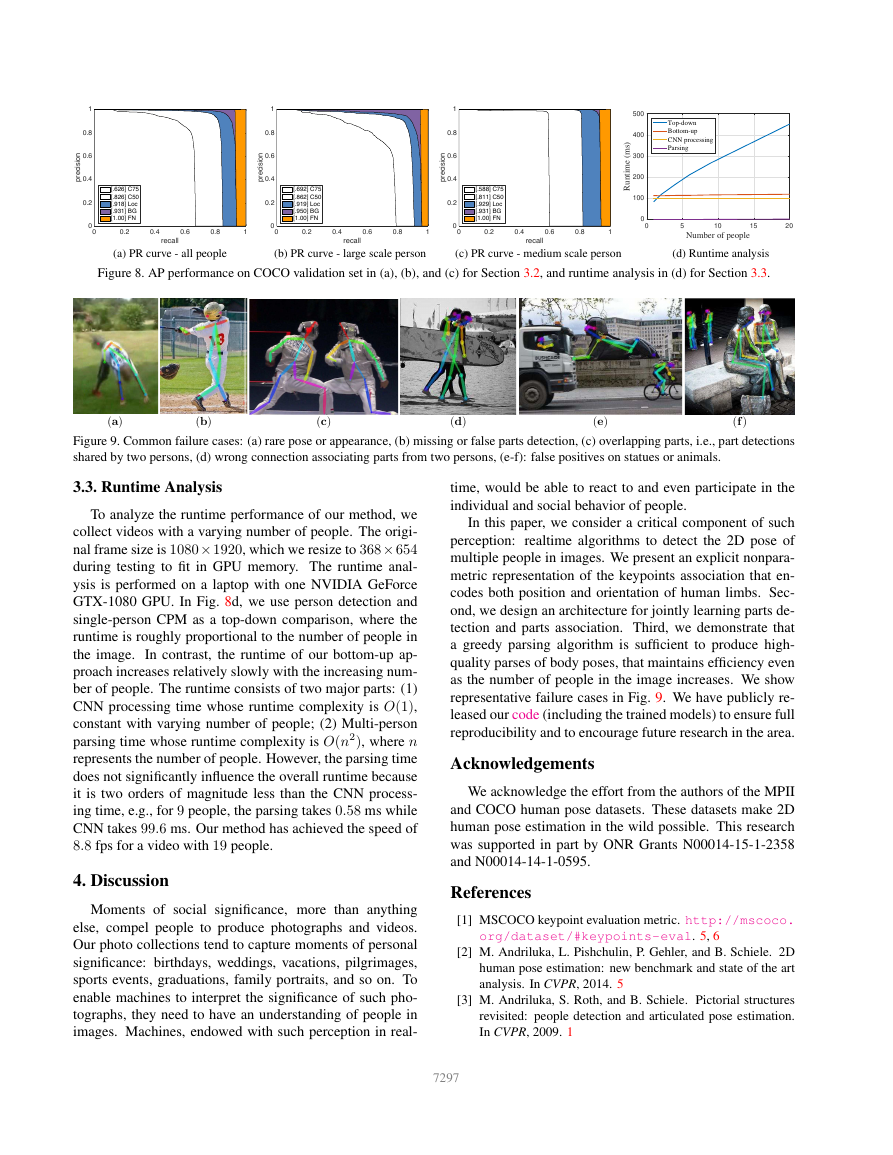
the performance of our bottom-up method. Fig. 8 shows a
breakdown of errors of our method on the COCO valida-
tion set. Most of the false positives come from imprecise
localization, other than background confusion. This indi-
cates there is more improvement space in capturing spatial
dependencies than in recognizing body parts appearances.
7296
�
i
i
n
o
s
c
e
r
p
1
0.8
0.6
0.4
0.2
0
0
[.626] C75
[.826] C50
[.918] Loc
[.931] BG
[1.00] FN
0.2
0.4
0.6
0.8
1
recall
i
i
n
o
s
c
e
r
p
1
0.8
0.6
0.4
0.2
0
0
[.692] C75
[.862] C50
[.919] Loc
[.950] BG
[1.00] FN
0.2
0.4
0.6
0.8
1
recall
i
i
n
o
s
c
e
r
p
1
0.8
0.6
0.4
0.2
0
0
500
400
300
200
100
)
s
m
(
e
m
i
t
n
u
R
0
0
Top-down
Bottom-up
CNN processing
Parsing
5
10
15
20
Number of people
[.588] C75
[.811] C50
[.929] Loc
[.931] BG
[1.00] FN
0.2
0.4
0.6
0.8
1
recall
(a) PR curve - all people
(b) PR curve - large scale person
(c) PR curve - medium scale person
(d) Runtime analysis
Figure 8. AP performance on COCO validation set in (a), (b), and (c) for Section 3.2, and runtime analysis in (d) for Section 3.3.
(a)
(b)
(c)
(d)
(e)
(f )
Figure 9. Common failure cases: (a) rare pose or appearance, (b) missing or false parts detection, (c) overlapping parts, i.e., part detections
shared by two persons, (d) wrong connection associating parts from two persons, (e-f): false positives on statues or animals.
3.3. Runtime Analysis
To analyze the runtime performance of our method, we
collect videos with a varying number of people. The origi-
nal frame size is 1080 × 1920, which we resize to 368 × 654
during testing to fit in GPU memory. The runtime anal-
ysis is performed on a laptop with one NVIDIA GeForce
GTX-1080 GPU. In Fig. 8d, we use person detection and
single-person CPM as a top-down comparison, where the
runtime is roughly proportional to the number of people in
the image. In contrast, the runtime of our bottom-up ap-
proach increases relatively slowly with the increasing num-
ber of people. The runtime consists of two major parts: (1)
CNN processing time whose runtime complexity is O(1),
constant with varying number of people; (2) Multi-person
parsing time whose runtime complexity is O(n2), where n
represents the number of people. However, the parsing time
does not significantly influence the overall runtime because
it is two orders of magnitude less than the CNN process-
ing time, e.g., for 9 people, the parsing takes 0.58 ms while
CNN takes 99.6 ms. Our method has achieved the speed of
8.8 fps for a video with 19 people.
4. Discussion
Moments of social significance, more than anything
else, compel people to produce photographs and videos.
Our photo collections tend to capture moments of personal
significance: birthdays, weddings, vacations, pilgrimages,
sports events, graduations, family portraits, and so on. To
enable machines to interpret the significance of such pho-
tographs, they need to have an understanding of people in
images. Machines, endowed with such perception in real-
time, would be able to react to and even participate in the
individual and social behavior of people.
In this paper, we consider a critical component of such
perception: realtime algorithms to detect the 2D pose of
multiple people in images. We present an explicit nonpara-
metric representation of the keypoints association that en-
codes both position and orientation of human limbs. Sec-
ond, we design an architecture for jointly learning parts de-
tection and parts association. Third, we demonstrate that
a greedy parsing algorithm is sufficient to produce high-
quality parses of body poses, that maintains efficiency even
as the number of people in the image increases. We show
representative failure cases in Fig. 9. We have publicly re-
leased our code (including the trained models) to ensure full
reproducibility and to encourage future research in the area.
Acknowledgements
We acknowledge the effort from the authors of the MPII
and COCO human pose datasets. These datasets make 2D
human pose estimation in the wild possible. This research
was supported in part by ONR Grants N00014-15-1-2358
and N00014-14-1-0595.
References
[1] MSCOCO keypoint evaluation metric. http://mscoco.
org/dataset/#keypoints-eval. 5, 6
[2] M. Andriluka, L. Pishchulin, P. Gehler, and B. Schiele. 2D
human pose estimation: new benchmark and state of the art
analysis. In CVPR, 2014. 5
[3] M. Andriluka, S. Roth, and B. Schiele. Pictorial structures
revisited: people detection and articulated pose estimation.
In CVPR, 2009. 1
7297
�
Figure 10. Results containing viewpoint and appearance variation, occlusion, crowding, contact, and other common imaging artifacts.
7298
�



 2023年江西萍乡中考道德与法治真题及答案.doc
 2012年重庆南川中考生物真题及答案.doc
 2013年江西师范大学地理学综合及文艺理论基础考研真题.doc
 2020年四川甘孜小升初语文真题及答案I卷.doc
 2020年注册岩土工程师专业基础考试真题及答案.doc
 2023-2024学年福建省厦门市九年级上学期数学月考试题及答案.doc
 2021-2022学年辽宁省沈阳市大东区九年级上学期语文期末试题及答案.doc
 2022-2023学年北京东城区初三第一学期物理期末试卷及答案.doc
 2018上半年江西教师资格初中地理学科知识与教学能力真题及答案.doc
 2012年河北国家公务员申论考试真题及答案-省级.doc
 2020-2021学年江苏省扬州市江都区邵樊片九年级上学期数学第一次质量检测试题及答案.doc
 2022下半年黑龙江教师资格证中学综合素质真题及答案.doc