Face Recognition with Python
Philipp Wagner
http://www.bytefish.de
July 18, 2012
Contents
1 Introduction
2 Face Recognition
2.1 Face Database
. . . . . . . . . . . . . . . . . . . . . . . . . . . . . . . . . . . . . . . .
2.1.1 Reading the images with Python . . . . . . . . . . . . . . . . . . . . . . . . . .
2.2 Eigenfaces . . . . . . . . . . . . . . . . . . . . . . . . . . . . . . . . . . . . . . . . . . .
2.2.1 Algorithmic Description . . . . . . . . . . . . . . . . . . . . . . . . . . . . . . .
2.2.2 Eigenfaces in Python . . . . . . . . . . . . . . . . . . . . . . . . . . . . . . . . .
. . . . . . . . . . . . . . . . . . . . . . . . . . . . . . . . . . . . . . . . . .
2.3.1 Algorithmic Description . . . . . . . . . . . . . . . . . . . . . . . . . . . . . . .
2.3.2 Fisherfaces in Python . . . . . . . . . . . . . . . . . . . . . . . . . . . . . . . .
2.3 Fisherfaces
3 Conclusion
1
Introduction
1
2
2
3
4
4
5
10
10
12
15
In this document I’ll show you how to implement the Eigenfaces [13] and Fisherfaces [3] method with
Python, so you’ll understand the basics of Face Recognition. All concepts are explained in detail, but a
basic knowledge of Python is assumed. Originally this document was a Guide to Face Recognition with
OpenCV. Since OpenCV now comes with the cv::FaceRecognizer, this document has been reworked
into the official OpenCV documentation at:
• http://docs.opencv.org/trunk/modules/contrib/doc/facerec/index.html
I am doing all this in my spare time and I simply can’t maintain two separate documents on the
same topic any more. So I have decided to turn this document into a guide on Face Recognition with
Python only. You’ll find the very detailed documentation on the OpenCV cv::FaceRecognizer at:
• FaceRecognizer - Face Recognition with OpenCV
– FaceRecognizer API
– Guide to Face Recognition with OpenCV
– Tutorial on Gender Classification
– Tutorial on Face Recognition in Videos
– Tutorial On Saving & Loading a FaceRecognizer
By the way you don’t need to copy and paste the code snippets, all code has been pushed into my
github repository:
• github.com/bytefish
• github.com/bytefish/facerecognition guide
Everything in here is released under a BSD license, so feel free to use it for your projects. You
are currently reading the Python version of the Face Recognition Guide, you can compile the GNU
Octave/MATLAB version with make octave.
1
�
2 Face Recognition
Face recognition is an easy task for humans. Experiments in [6] have shown, that even one to three
day old babies are able to distinguish between known faces. So how hard could it be for a computer?
It turns out we know little about human recognition to date. Are inner features (eyes, nose, mouth)
or outer features (head shape, hairline) used for a successful face recognition? How do we analyze an
image and how does the brain encode it? It was shown by David Hubel and Torsten Wiesel, that our
brain has specialized nerve cells responding to specific local features of a scene, such as lines, edges,
angles or movement. Since we don’t see the world as scattered pieces, our visual cortex must somehow
combine the different sources of information into useful patterns. Automatic face recognition is all
about extracting those meaningful features from an image, putting them into a useful representation
and performing some kind of classification on them.
Face recognition based on the geometric features of a face is probably the most intuitive approach to
face recognition. One of the first automated face recognition systems was described in [9]: marker
points (position of eyes, ears, nose, ...) were used to build a feature vector (distance between the
points, angle between them, ...). The recognition was performed by calculating the euclidean distance
between feature vectors of a probe and reference image. Such a method is robust against changes in
illumination by its nature, but has a huge drawback: the accurate registration of the marker points
is complicated, even with state of the art algorithms. Some of the latest work on geometric face
recognition was carried out in [4]. A 22-dimensional feature vector was used and experiments on
large datasets have shown, that geometrical features alone don’t carry enough information for face
recognition.
The Eigenfaces method described in [13] took a holistic approach to face recognition: A facial image is
a point from a high-dimensional image space and a lower-dimensional representation is found, where
classification becomes easy. The lower-dimensional subspace is found with Principal Component
Analysis, which identifies the axes with maximum variance. While this kind of transformation is
optimal from a reconstruction standpoint, it doesn’t take any class labels into account. Imagine a
situation where the variance is generated from external sources, let it be light. The axes with maximum
variance do not necessarily contain any discriminative information at all, hence a classification becomes
impossible. So a class-specific projection with a Linear Discriminant Analysis was applied to face
recognition in [3]. The basic idea is to minimize the variance within a class, while maximizing the
variance between the classes at the same time (Figure 1).
Recently various methods for a local feature extraction emerged. To avoid the high-dimensionality of
the input data only local regions of an image are described, the extracted features are (hopefully) more
robust against partial occlusion, illumation and small sample size. Algorithms used for a local feature
extraction are Gabor Wavelets ([14]), Discrete Cosinus Transform ([5]) and Local Binary Patterns
([1, 11, 12]). It’s still an open research question how to preserve spatial information when applying a
local feature extraction, because spatial information is potentially useful information.
2.1 Face Database
I don’t want to do a toy example here. We are doing face recognition, so you’ll need some face
images! You can either create your own database or start with one of the available databases, face-
rec.org/databases gives an up-to-date overview. Three interesting databases are1:
AT&T Facedatabase The AT&T Facedatabase, sometimes also known as ORL Database of Faces,
contains ten different images of each of 40 distinct subjects. For some subjects, the images were
taken at different times, varying the lighting, facial expressions (open / closed eyes, smiling /
not smiling) and facial details (glasses / no glasses). All the images were taken against a dark
homogeneous background with the subjects in an upright, frontal position (with tolerance for
some side movement).
Yale Facedatabase A The AT&T Facedatabase is good for initial tests, but it’s a fairly easy
database. The Eigenfaces method already has a 97% recognition rate, so you won’t see any
improvements with other algorithms. The Yale Facedatabase A is a more appropriate dataset
for initial experiments, because the recognition problem is harder. The database consists of
15 people (14 male, 1 female) each with 11 grayscale images sized 320 × 243 pixel. There are
1Parts of the description are quoted from face-rec.org.
2
�
changes in the light conditions (center light, left light, right light), facial expressions (happy,
normal, sad, sleepy, surprised, wink) and glasses (glasses, no-glasses).
The original images are not cropped or aligned.
src/py/crop_face.py, that does the job for you.
I’ve prepared a Python script available in
Extended Yale Facedatabase B The Extended Yale Facedatabase B contains 2414 images of 38
different people in its cropped version. The focus is on extracting features that are robust to
illumination, the images have almost no variation in emotion/occlusion/. . .. I personally think,
that this dataset is too large for the experiments I perform in this document, you better use
the AT&T Facedatabase. A first version of the Yale Facedatabase B was used in [3] to see how
the Eigenfaces and Fisherfaces method (section 2.3) perform under heavy illumination changes.
[10] used the same setup to take 16128 images of 28 people. The Extended Yale Facedatabase
B is the merge of the two databases, which is now known as Extended Yalefacedatabase B.
The face images need to be stored in a folder hierachy similar to //.. The AT&T Facedatabase for example comes in such a hierarchy, see Listing 1.
Listing 1:
| - - 1. pgm
| - - ...
| - - 10. pgm
p h i l i p p @ m a n g o :~/ facerec / data / at$ tree
.
| - - README
| - - s1
|
|
|
| - - s2
|
|
|
...
| - - s40
|
|
|
| - - 1. pgm
| - - ...
| - - 10. pgm
| - - 1. pgm
| - - ...
| - - 10. pgm
2.1.1 Reading the images with Python
The function in Listing 2 can be used to read in the images for each subfolder of a given directory.
Each directory is given a unique (integer) label, you probably want to store the folder name as well.
The function returns the images and the corresponding classes. This function is really basic and
there’s much to enhance, but it does its job.
Listing 2: src/py/tinyfacerec/util.py
def r e a d _ i m a g e s ( path , sz = None ) :
c = 0
X , y = [] , []
for dirname , dirnames , f i l e n a m e s in os . walk ( path ) :
for s u b d i r n a m e in d i r n a m e s :
s u b j e c t _ p a t h = os . path . join ( dirname , s u b d i r n a m e )
for f i l e n a m e in os . listdir ( s u b j e c t _ p a t h ) :
try :
im = Image . open ( os . path . join ( subject_path , f i l e n a m e ) )
im = im . convert ( " L " )
# resize to given size ( if given )
if ( sz is not None ) :
im = im . resize ( sz , Image . A N T I A L I A S )
X . append ( np . asarray ( im , dtype = np . uint8 ) )
y . append ( c )
except IOError :
print " I / O error ({0}) : {1} " . format ( errno , s t r e r r o r )
except :
print " U n e x p e c t e d error : " , sys . e x c _ i n f o () [0]
raise
c = c +1
return [X , y ]
3
�
2.2 Eigenfaces
The problem with the image representation we are given is its high dimensionality. Two-dimensional
p × q grayscale images span a m = pq-dimensional vector space, so an image with 100 × 100 pixels
lies in a 10, 000-dimensional image space already. That’s way too much for any computations, but are
all dimensions really useful for us? We can only make a decision if there’s any variance in data, so
what we are looking for are the components that account for most of the information. The Principal
Component Analysis (PCA) was independently proposed by Karl Pearson (1901) and Harold Hotelling
(1933) to turn a set of possibly correlated variables into a smaller set of uncorrelated variables. The
idea is that a high-dimensional dataset is often described by correlated variables and therefore only a
few meaningful dimensions account for most of the information. The PCA method finds the directions
with the greatest variance in the data, called principal components.
2.2.1 Algorithmic Description
Let X = {x1, x2, . . . , xn} be a random vector with observations xi ∈ Rd.
1. Compute the mean µ
µ =
1
n
xi
n
i=1
2. Compute the the Covariance Matrix S
S =
1
n
n
i=1
(xi − µ)(xi − µ)T
3. Compute the eigenvalues λi and eigenvectors vi of S
Svi = λivi, i = 1, 2, . . . , n
(1)
(2)
(3)
4. Order the eigenvectors descending by their eigenvalue. The k principal components are the
eigenvectors corresponding to the k largest eigenvalues.
The k principal components of the observed vector x are then given by:
where W = (v1, v2, . . . , vk). The reconstruction from the PCA basis is given by:
y = W T (x − µ)
The Eigenfaces method then performs face recognition by:
x = W y + µ
(4)
(5)
1. Projecting all training samples into the PCA subspace (using Equation 4).
2. Projecting the query image into the PCA subspace (using Listing 5).
3. Finding the nearest neighbor between the projected training images and the projected query
image.
Still there’s one problem left to solve. Imagine we are given 400 images sized 100 × 100 pixel. The
Principal Component Analysis solves the covariance matrix S = XX T , where size(X) = 10000 × 400
in our example. You would end up with a 10000× 10000 matrix, roughly 0.8GB. Solving this problem
isn’t feasible, so we’ll need to apply a trick. From your linear algebra lessons you know that a M × N
matrix with M > N can only have N − 1 non-zero eigenvalues. So it’s possible to take the eigenvalue
decomposition S = X T X of size N xN instead:
and get the original eigenvectors of S = XX T with a left multiplication of the data matrix:
X T Xvi = λivi
XX T (Xvi) = λi(Xvi)
(6)
(7)
The resulting eigenvectors are orthogonal, to get orthonormal eigenvectors they need to be normalized
to unit length. I don’t want to turn this into a publication, so please look into [7] for the derivation
and proof of the equations.
4
�
2.2.2 Eigenfaces in Python
We’ve already seen, that the Eigenfaces and Fisherfaces method expect a data matrix with observations
by row (or column if you prefer it). Listing 3 defines two functions to reshape a list of multi-dimensional
data into a data matrix. Note, that all samples are assumed to be of equal size.
Listing 3: src/py/tinyfacerec/util.py
def a s R o w M a t r i x ( X ) :
if len ( X ) == 0:
return np . array ([])
mat = np . empty ((0 , X [0]. size ) , dtype = X [0]. dtype )
for row in X :
mat = np . vstack (( mat , np . asarray ( row ) . reshape (1 , -1) ) )
return mat
def a s C o l u m n M a t r i x ( X ) :
if len ( X ) == 0:
return np . array ([])
mat = np . empty (( X [0]. size , 0) , dtype = X [0]. dtype )
for col in X :
mat = np . hstack (( mat , np . asarray ( col ) . reshape ( -1 ,1) ) )
return mat
Translating the PCA from the algorithmic description of section 2.2.1 to Python is almost trivial.
Don’t copy and paste from this document, the source code is available in folder src/py/tinyfacerec
. Listing 4 implements the Principal Component Analysis given by Equation 1, 2 and 3.
It also
implements the inner-product PCA formulation, which occurs if there are more dimensions than
samples. You can shorten this code, I just wanted to point out how it works.
Listing 4: src/py/tinyfacerec/subspace.py
def pca (X , y , n u m _ c o m p o n e n t s =0) :
[n , d ] = X . shape
if ( n u m _ c o m p o n e n t s <= 0) or ( num_components > n ) :
n u m _ c o m p o n e n t s = n
mu = X . mean ( axis =0)
X = X - mu
if n > d :
C = np . dot ( X .T , X )
[ eigenvalues , e i g e n v e c t o r s ] = np . linalg . eigh ( C )
else :
C = np . dot (X , X . T )
[ eigenvalues , e i g e n v e c t o r s ] = np . linalg . eigh ( C )
e i g e n v e c t o r s = np . dot ( X .T , e i g e n v e c t o r s )
for i in xrange ( n ) :
e i g e n v e c t o r s [: , i ] = e i g e n v e c t o r s [: , i ]/ np . linalg . norm ( e i g e n v e c t o r s [: , i ])
# or simply perform an economy size d e c o m p o s i t i o n
# eigenvectors , eigenvalues , v a r i a n c e = np . linalg . svd ( X .T , f u l l _ m a t r i c e s = False )
# sort e i g e n v e c t o r s d e s c e n d i n g by their e i g e n v a l u e
idx = np . argsort ( - e i g e n v a l u e s )
e i g e n v a l u e s = e i g e n v a l u e s [ idx ]
e i g e n v e c t o r s = e i g e n v e c t o r s [: , idx ]
# select only n u m _ c o m p o n e n t s
e i g e n v a l u e s = e i g e n v a l u e s [0: n u m _ c o m p o n e n t s ]. copy ()
e i g e n v e c t o r s = e i g e n v e c t o r s [: ,0: n u m _ c o m p o n e n t s ]. copy ()
return [ eigenvalues , eigenvectors , mu ]
The observations are given by row, so the projection in Equation 4 needs to be rearranged a little:
Listing 5: src/py/tinyfacerec/subspace.py
def project (W , X , mu = None ) :
if mu is None :
return np . dot (X , W )
return np . dot ( X - mu , W )
The same applies to the reconstruction in Equation 5:
Listing 6: src/py/tinyfacerec/subspace.py
5
�
def r e c o n s t r u c t (W , Y , mu = None ) :
if mu is None :
return np . dot (Y , W . T )
return np . dot (Y , W . T ) + mu
Now that everything is defined it’s time for the fun stuff. The face images are read with Listing 2
and then a full PCA (see Listing 4) is performed. I’ll use the great matplotlib library for plotting in
Python, please install it if you haven’t done already.
Listing 7: src/py/scripts/example pca.py
import sys
# append t i n y f a c e r e c to module search path
sys . path . append ( " .. " )
# import numpy and m a t p l o t l i b c o l o r m a p s
import numpy as np
# import t i n y f a c e r e c modules
from t i n y f a c e r e c . s u b s p a c e import pca
from t i n y f a c e r e c . util import normalize , asRowMatrix , r e a d _ i m a g e s
from t i n y f a c e r e c . visual import subplot
# read images
[X , y ] = r e a d _ i m a g e s ( " / home / philipp / facerec / data / at " )
# perform a full pca
[D , W , mu ] = pca ( a s R o w M a t r i x ( X ) , y )
That’s it already. Pretty easy, no? Each principal component has the same length as the original
image, thus it can be displayed as an image. [13] referred to these ghostly looking faces as Eigenfaces,
that’s where the Eigenfaces method got its name from. We’ll now want to look at the Eigenfaces,
but first of all we need a method to turn the data into a representation matplotlib understands.
The eigenvectors we have calculated can contain negative values, but the image data is excepted as
unsigned integer values in the range of 0 to 255. So we need a function to normalize the data first
(Listing 8):
def n o r m a l i z e (X , low , high , dtype = None ) :
Listing 8: src/py/tinyfacerec/util.py
X = np . asarray ( X )
minX , maxX = np . min ( X ) , np . max ( X )
# n o r m a l i z e to [ 0 . . . 1 ] .
X = X - float ( minX )
X = X / float (( maxX - minX ) )
# scale to [ low ... high ].
X = X * ( high - low )
X = X + low
if dtype is None :
return np . asarray ( X )
return np . asarray (X , dtype = dtype )
In Python we’ll then define a subplot method (see src/py/tinyfacerec/visual.py) to simplify the
plotting. The method takes a list of images, a title, color scale and finally generates a subplot:
Listing 9: src/py/tinyfacerec/visual.py
import numpy as np
import m a t p l o t l i b . pyplot as plt
import m a t p l o t l i b . cm as cm
def c r e a t e _ f o n t ( f o n t n a m e = ’ Tahoma ’ , f o n t s i z e =10) :
return { ’ f o n t n a m e ’: fontname , ’ f o n t s i z e ’: f o n t s i z e }
def subplot ( title , images , rows , cols , sptitle = " subplot " , s p t i t l e s =[] , c o l o r m a p = cm .
gray , t i c k s _ v i s i b l e = True , f i l e n a m e = None ) :
fig = plt . figure ()
# main title
fig . text (.5 , .95 , title , h o r i z o n t a l a l i g n m e n t = ’ center ’)
for i in xrange ( len ( images ) ) :
ax0 = fig . a d d _ s u b p l o t ( rows , cols ,( i +1) )
plt . setp ( ax0 . g e t _ x t i c k l a b e l s () , visible = False )
plt . setp ( ax0 . g e t _ y t i c k l a b e l s () , visible = False )
6
�
if len ( s p t i t l e s ) == len ( images ) :
plt . title ( " % s #% s " % ( sptitle , str ( s p t i t l e s [ i ]) ) , c r e a t e _ f o n t ( ’ Tahoma ’ ,10) )
else :
plt . title ( " % s #% d " % ( sptitle , ( i +1) ) , c r e a t e _ f o n t ( ’ Tahoma ’ ,10) )
plt . imshow ( np . asarray ( images [ i ]) , cmap = c o l o r m a p )
if f i l e n a m e is None :
plt . show ()
else :
fig . savefig ( f i l e n a m e )
This simplified the Python script in Listing 10 to:
Listing 10: src/py/scripts/example pca.py
import m a t p l o t l i b . cm as cm
# turn the first ( at most ) 16 e i g e n v e c t o r s into g r a y s c a l e
# images ( note : e i g e n v e c t o r s are stored by column !)
E = []
for i in xrange ( min ( len ( X ) , 16) ) :
e = W [: , i ]. reshape ( X [0]. shape )
E . append ( n o r m a l i z e (e ,0 ,255) )
# plot them and store the plot to " p y t h o n _ e i g e n f a c e s . pdf "
subplot ( title = " E i g e n f a c e s AT & T F a c e d a t a b a s e " , images =E , rows =4 , cols =4 , sptitle = "
E i g e n f a c e " , c o l o r m a p = cm . jet , f i l e n a m e = " p y t h o n _ p c a _ e i g e n f a c e s . png " )
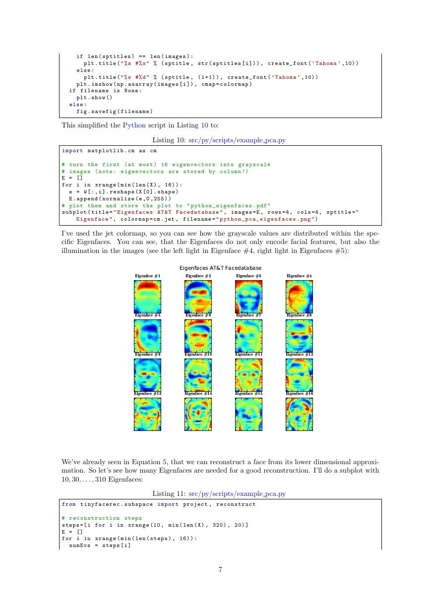
I’ve used the jet colormap, so you can see how the grayscale values are distributed within the spe-
cific Eigenfaces. You can see, that the Eigenfaces do not only encode facial features, but also the
illumination in the images (see the left light in Eigenface #4, right light in Eigenfaces #5):
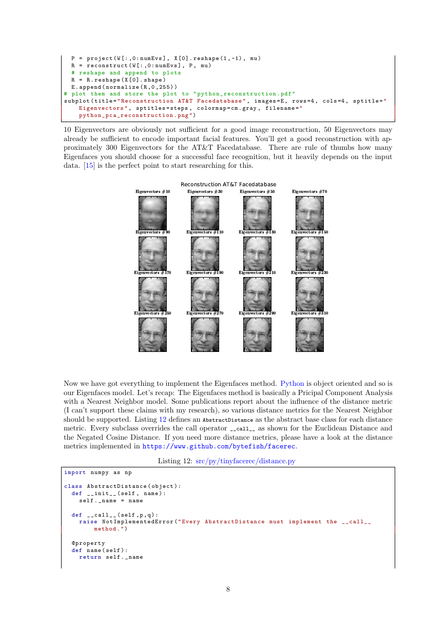
We’ve already seen in Equation 5, that we can reconstruct a face from its lower dimensional approxi-
mation. So let’s see how many Eigenfaces are needed for a good reconstruction. I’ll do a subplot with
10, 30, . . . , 310 Eigenfaces:
Listing 11: src/py/scripts/example pca.py
from t i n y f a c e r e c . s u b s p a c e import project , r e c o n s t r u c t
# r e c o n s t r u c t i o n steps
steps =[ i for i in xrange (10 , min ( len ( X ) , 320) , 20) ]
E = []
for i in xrange ( min ( len ( steps ) , 16) ) :
numEvs = steps [ i ]
7
Eigenface #1Eigenface #2Eigenface #3Eigenface #4Eigenface #5Eigenface #6Eigenface #7Eigenface #8Eigenface #9Eigenface #10Eigenface #11Eigenface #12Eigenface #13Eigenface #14Eigenface #15Eigenface #16Eigenfaces AT&T Facedatabase�
P = project ( W [: ,0: numEvs ] , X [0]. reshape (1 , -1) , mu )
R = r e c o n s t r u c t ( W [: ,0: numEvs ] , P , mu )
# reshape and append to plots
R = R . reshape ( X [0]. shape )
E . append ( n o r m a l i z e (R ,0 ,255) )
# plot them and store the plot to " p y t h o n _ r e c o n s t r u c t i o n . pdf "
subplot ( title = " R e c o n s t r u c t i o n AT & T F a c e d a t a b a s e " , images =E , rows =4 , cols =4 , sptitle = "
E i g e n v e c t o r s " , s p t i t l e s = steps , c o l o r m a p = cm . gray , f i l e n a m e = "
p y t h o n _ p c a _ r e c o n s t r u c t i o n . png " )
10 Eigenvectors are obviously not sufficient for a good image reconstruction, 50 Eigenvectors may
already be sufficient to encode important facial features. You’ll get a good reconstruction with ap-
proximately 300 Eigenvectors for the AT&T Facedatabase. There are rule of thumbs how many
Eigenfaces you should choose for a successful face recognition, but it heavily depends on the input
data. [15] is the perfect point to start researching for this.
Now we have got everything to implement the Eigenfaces method. Python is object oriented and so is
our Eigenfaces model. Let’s recap: The Eigenfaces method is basically a Pricipal Component Analysis
with a Nearest Neighbor model. Some publications report about the influence of the distance metric
(I can’t support these claims with my research), so various distance metrics for the Nearest Neighbor
should be supported. Listing 12 defines an AbstractDistance as the abstract base class for each distance
metric. Every subclass overrides the call operator __call__ as shown for the Euclidean Distance and
the Negated Cosine Distance. If you need more distance metrics, please have a look at the distance
metrics implemented in https://www.github.com/bytefish/facerec.
Listing 12: src/py/tinyfacerec/distance.py
import numpy as np
class A b s t r a c t D i s t a n c e ( object ) :
def _ _ i n i t _ _ ( self , name ) :
self . _name = name
def _ _ c a l l _ _ ( self ,p , q ) :
raise N o t I m p l e m e n t e d E r r o r ( " Every A b s t r a c t D i s t a n c e must i m p l e m e n t the _ _ c a l l _ _
method . " )
@ p r o p e r t y
def name ( self ) :
return self . _name
8
Eigenvectors #10Eigenvectors #30Eigenvectors #50Eigenvectors #70Eigenvectors #90Eigenvectors #110Eigenvectors #130Eigenvectors #150Eigenvectors #170Eigenvectors #190Eigenvectors #210Eigenvectors #230Eigenvectors #250Eigenvectors #270Eigenvectors #290Eigenvectors #310Reconstruction AT&T Facedatabase�




 2023年江西萍乡中考道德与法治真题及答案.doc
 2012年重庆南川中考生物真题及答案.doc
 2013年江西师范大学地理学综合及文艺理论基础考研真题.doc
 2020年四川甘孜小升初语文真题及答案I卷.doc
 2020年注册岩土工程师专业基础考试真题及答案.doc
 2023-2024学年福建省厦门市九年级上学期数学月考试题及答案.doc
 2021-2022学年辽宁省沈阳市大东区九年级上学期语文期末试题及答案.doc
 2022-2023学年北京东城区初三第一学期物理期末试卷及答案.doc
 2018上半年江西教师资格初中地理学科知识与教学能力真题及答案.doc
 2012年河北国家公务员申论考试真题及答案-省级.doc
 2020-2021学年江苏省扬州市江都区邵樊片九年级上学期数学第一次质量检测试题及答案.doc
 2022下半年黑龙江教师资格证中学综合素质真题及答案.doc