Regression Shrinkage and Selection via the Lasso
Author(s): Robert Tibshirani
Source: Journal of the Royal Statistical Society. Series B (Methodological), Vol. 58, No. 1
(1996), pp. 267-288
Published by: Blackwell Publishing for the Royal Statistical Society
Stable URL: http://www.jstor.org/stable/2346178 .
Accessed: 05/01/2011 02:51
Your use of the JSTOR archive indicates your acceptance of JSTOR's Terms and Conditions of Use, available at .
http://www.jstor.org/page/info/about/policies/terms.jsp. JSTOR's Terms and Conditions of Use provides, in part, that unless
you have obtained prior permission, you may not download an entire issue of a journal or multiple copies of articles, and you
may use content in the JSTOR archive only for your personal, non-commercial use.
Please contact the publisher regarding any further use of this work. Publisher contact information may be obtained at .
http://www.jstor.org/action/showPublisher?publisherCode=black. .
Each copy of any part of a JSTOR transmission must contain the same copyright notice that appears on the screen or printed
page of such transmission.
JSTOR is a not-for-profit service that helps scholars, researchers, and students discover, use, and build upon a wide range of
content in a trusted digital archive. We use information technology and tools to increase productivity and facilitate new forms
of scholarship. For more information about JSTOR, please contact support@jstor.org.
Blackwell Publishing and Royal Statistical Society are collaborating with JSTOR to digitize, preserve and
extend access to Journal of the Royal Statistical Society. Series B (Methodological).
http://www.jstor.org
�
J. R. Statist. Soc. B (1996)
58, No. 1, pp. 267-288
Regression Shrinkage and Selection via the Lasso
By ROBERT TIBSHIRANIt
University of Toronto, Canada
[Received January 1994. Revised January 1995]
SUMMARY
We propose a new method for estimation in linear models. The 'lasso' minimizes the
residual sum of squares subject to the sum of the absolute value of the coefficients being less
than a constant. Because of the nature of this constraint it tends to produce some
coefficients that are exactly 0 and hence gives interpretable models. Our simulation studies
suggest that the lasso enjoys some of the favourable properties of both subset selection and
ridge regression. It produces interpretable models like subset selection and exhibits the
stability of ridge regression. There is also an interesting relationship with recent work in
adaptive function estimation by Donoho and Johnstone. The lasso idea is quite general and
can be applied in a variety of statistical models: extensions to generalized regression models
and tree-based models are briefly described.
Keywords: QUADRATIC PROGRAMMING; REGRESSION; SHRINKAGE; SUBSET SELECTION
1. INTRODUCTION
(x,..
Consider the usual regression situation: we have data (xi, yi), i = 1, 2, . . ., N, where
., xP)T and yi are the regressors and response for the ith observation.
x=
The ordinary least squares (OLS) estimates are obtained by minimizing the residual
squared error. There are two reasons why the data analyst is often not satisfied with
the OLS estimates. The first is prediction accuracy: the OLS estimates often have low
bias but large variance; prediction accuracy can sometimes be improved by shrinking
or setting to 0 some coefficients. By doing so we sacrifice a little bias to reduce the
variance of the predicted values and hence may improve the overall prediction
accuracy. The second reason is interpretation. With a large number of predictors, we
often would like to determine a smaller subset that exhibits the strongest effects.
The two standard techniques for improving the OLS estimates, subset selection
and ridge regression, both have drawbacks. Subset selection provides interpretable
models but can be extremely variable because it is a discrete process - regressors are
either retained or dropped from the model. Small changes in the data can result in
very different models being selected and this can reduce its prediction accuracy.
Ridge regression is a continuous process that shrinks coefficients and hence is more
stable: however, it does not set any coefficients to 0 and hence does not give an easily
interpretable model.
We propose a new technique, called the lasso, for 'least absolute shrinkage and
selection operator'. It shrinks some coefficients and sets others to 0, and hence tries to
retain the good features of both subset selection and ridge regression.
tAddress for correspondence: Department of Preventive Medicine and Biostatistics, and Department of Statistics,
University of Toronto, 12 Queen's Park Crescent West, Toronto, Ontario, M5S 1A8, Canada.
E-mail: tibs@utstat.toronto.edu
? 1996 Royal Statistical Society
0035-9246/96/58267
�
268
TIBSHIRANI
[No. 1,
In Section 2 we define the lasso and look at some special cases. A real data example is
given in Section 3, while in Section 4 we discuss methods for estimation of prediction error
and the lasso shrinkage parameter. A Bayes model for the lasso is briefly mentioned in
Section 5. We describe the lasso algorithm in Section 6. Simulation studies are described in
Section 7. Sections 8 and 9 discuss extensions to generalized regression models and other
problems. Some results on soft thresholding and their relationship to the lasso are
discussed in Section 10, while Section 11 contains a summary and some discussion.
2. THE LASSO
2.1. Definition
Suppose that we have data (xi, yi), i = 1, 2, . . ., N, where xi = (xi, .. . X, )T are
the predictor variables and yi are the responses. As in the usual regression set-up, we
assume either that the observations are independent or that the yis are conditionally
independent given the xys. We assume that the xy are standardized so that 2ixyl/N
?, Eix2/N
Letting ,3 = (PI, . . ., pp)T, the lasso estimate (&, /3) is defined by
=1.
(&3)=argminf
(Yi-a-L 5 1X)2)} subject toZlfBll t.
(1)
Here t > 0 is a tuning parameter. Now, for all t, the solution for a is & y. We can
assume without loss of generality that j 0 0 and hence omit a.
Computation of the solution to equation (1) is a quadratic programming problem
with linear inequality constraints. We describe some efficient and stable algorithms
for this problem in Section 6.
The parameter t > 0 controls the amount of shrinkage that is a,pplied to the
estimates. Let fl be the full least squares estimates and let to SIfl. Values of
t < to will cause shrinkage of the solutions towards 0, and some coefficients may be
exactly equal to 0. For example, if t = to/2, the effect will be roughly similar to
finding the best subset of size p/2. Note also that the design matrix need not be of full
rank. In Section 4 we give some data-based methods for estimation of t.
The motivation for the lasso came from an interesting proposal of Breiman (1993).
Breiman's non-negative garotte minimizes
N
E
(Yi- -E
2
x)
subject to Cj > 0, E Cj s t.
(2)
The garotte starts with the OLS estimates and shrinks them by non-negative factors
whose sum is constrained. In extensive simulation studies, Breiman showed that the
garotte has consistently lower prediction error than subset selection and is
competitive with ridge regression except when the true model has many small non-
zero coefficients.
A drawback of the garotte is that its solution depends on both the sign and the
magnitude of the OLS estimates. In overfit or highly correlated settings where the
OLS estimates behave poorly, the garotte may suffer as a result. In contrast, the lasso
avoids the explicit use of the OLS estimates.
�
1996]
REGRESSION SHRINKAGE AND SELECTION
269
Frank and Friedman (1993) proposed using a bound on the Lq-norm of the
parameters, where q is some number greater than or equal to 0; the lasso corresponds
to q = 1. We discuss this briefly in Section 10.
2.2. Orthonormal Design Case
Insight about the nature of the shrinkage can be gleaned from the orthonormal
design case. Let X be the n x p design matrix with iUth entry xij, and suppose that
XTX = I, the identity matrix.
The solutions to equation (1) are easily shown to be
pf = sign (1 ) (I6j -j y)I
(3)
where y is determined by the condition 2filjl = t. Interestingly, this has exactly the
same form as the soft shrinkage proposals of Donoho and Johnstone (1994) and
Donoho et al. (1995), applied to wavelet coefficients in the context of function
estimation. The connection between soft shrinkage and a minimum LI-norm penalty
was also pointed out by Donoho et al. (1992) for non-negative parameters in the
context of signal or image recovery. We elaborate more on this connection in Section
10.
In the orthonormal design case, best subset selection of size k reduces to choosing
in absolute value and setting the rest to 0. For some choice
l if 1,871 > X and to 0 otherwise. Ridge
the k largest coefficients
of X this is equivalent to setting fi,
regression minimizes
N
E Yi -
2
flxyj +A
2
P,2
or, equivalently, minimizes
?E (Yi-4jx,)
subject to fi) < t
(4)
The ridge solutions are
1 ^
where y depends on X or t. The garotte estimates are
t
P A2 )
t
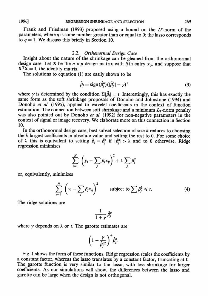
Fig. 1 shows the fonn of these functions. Ridge regression scales the coefficients by
a constant factor, whereas the lasso translates by a constant factor, truncating at 0.
The garotte function is very similar to the lasso, with less shrinkage for larger
coefficients. As our simulations will show, the differences between the lasso and
garotte can be large when the design is not orthogonal.
�
270
TIBSHIRANI
[No. 1,
2.3. Geometry of Lasso
It is clear from Fig. 1 why the lasso will often produce coefficients that are exactly
0. Why does this happen in the general (non-orthogonal) setting? And why does it
not occur with ridge regression, which uses the constraint ? fl2 K t rather than
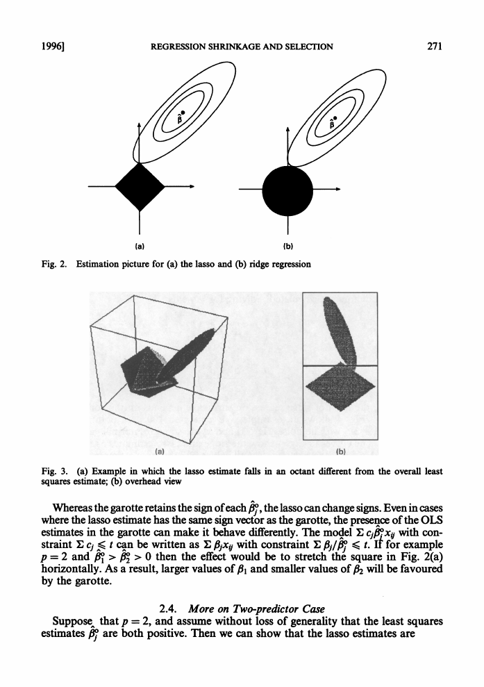
Elpl < t? Fig. 2 provides some insight for the case p = 2.
6jXij)2 equals the quadratic function
The criterion E1
(y,-
(,3-p
0) X
( X-
0)
(plus a constant). The elliptical contours of this function are shown by the full curves
in Fig. 2(a); they are centred at the OLS estimates; the constraint region is the rotated
square. The lasso solution is the first place that the contours touch the square, and
this will sometimes occur at a corner, corresponding to a zero coefficient. The picture
for ridge regression is shown in Fig. 2(b): there are no corners for the contours to hit
and hence zero solutions will rarely result.
An interesting question emerges from this picture: can the signs of the lasso
estimates be different from those of the least squares estimates ,j?? Since the variables
are standardized, when p = 2 the principal axes of the contours are at + 450 to the
co-ordinate axes, and we can show that the contours must contact the square in the
same quadrant that contains fi. However, when p > 2 and there is at least moderate
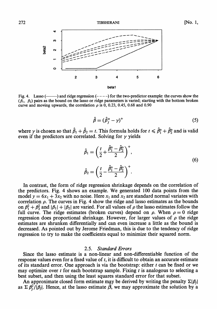
correlation in the data, this need not be true. Fig. 3 shows an example in three
dimensions. The view in Fig. 3(b) confirms that the ellipse touches the constraint
region in an octant different from the octant in which its centre lies.
N
N
LN
o
1
2
3
4
5
0
1
2
3
4
5
beta
(a)
beta
(b)
N
0
1
2
3
4
5
0
1
2
3
4
5
beta
(c)
beta
(d)
Fig. 1. (a) Subset regression, (b) ridge regression, (c) the lasso and (d) the garotte:
coefficient shrinkage in the orthonormal design case; ..........., 45?-line for reference
, form of
�
1996]
REGRESSION SHRINKAGE AND SELECTION
271
(a)
(b)
Fig. 2. Estimation picture for (a) the lasso and (b) ridge regression
(a)
lb)
Fig. 3. (a) Example in which the lasso estimate falls in an octant different from the overall least
squares estimate; (b) overhead view
Whereas the garotte retains the sign of each &, the lasso can change signs. Even in cases
where the lasso estimate has the same sign vector as the garotte, the presence of the OLS
estimates in the garotte can make it behave differently. The modjel E cj,fixy with con-
straint E Cj ^S t can be written as E fi1xy with constraint I fij/j
t. it for example
p = 2 and fil > 2 > 0 then the effect would be to stretch the square in Fig. 2(a)
horizontally. As a result, larger values of PI and smaller values of P2 will be favoured
by the garotte.
0
SupposeX that p = 2, and assume without loss of generality that the least squares
estimates P7 are both positive. Then we can show that the lasso estimates are
2.4. More on Two-predictor Case
�
272
TIBSHIRANI
[No. 1,
C%J)
2
3
4
5
6
betal
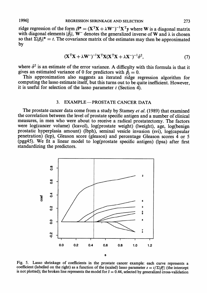
) and ridge regression ----) for the two-predictor example: the curves show the
Fig. 4. Lasso (
(P1, P2) pairs as the bound on the lasso or ridge parameters is varied; starting with the bottom broken
curve and moving upwards, the correlation p is 0, 0.23, 0.45, 0.68 and 0.90
(5)
where y is chosen so that ,81 + ,82 = t. This formula holds for t M l + 820 and is valid
even if the predictors are correlated. Solving for y yields
= (fO - Y)
(2
2
(6)
In contrast, the form of ridge regression shrinkage depends on the correlation of
the predictors. Fig. 4 shows an example. We generated 100 data points from the
model y = 6x1 + 3x2 with no noise. Here xl and x2 are standard normal variates with
correlation p. The curves in Fig. 4 show the ridge and lasso estimates as the bounds
on 216 + ,22 and 1fl1 I + 1f821 are varied. For all values of p the lasso estimates follow the
full curve. The ridge estimates (broken curves) depend on p. When p = 0 ridge
regression does proportional shrinkage. However, for larger values of p the ridge
and can even increase a little as the bound is
estimates are shrunken differentially
decreased. As pointed out by Jerome Friedman, this is due to the tendency of ridge
regression to try to make the coefficients equal to minimize their squared norm.
2.5. Standard Errors
Since the lasso estimate is a non-linear and non-differentiable
function of the
response values even for a fixed value of t, it is difficult to obtain an accurate estimate
of its standard error. One approach is via the bootstrap: either t can be fixed or we
may optimize over t for each bootstrap sample. Fixing t is analogous to selecting a
best subset, and then using the least squares standard error for that subset.
An approximate closed form estimate may be derived by writing the penalty Elfilj
as E ,6/lflfI. Hence, at the lasso estimate /, we may approximate the solution by a
�
REGRESSION SHRINKAGE AND SELECTION
1996]
ridge regression of the form /* = (XTX + W-)-lXTy where W is a diagonal matrix
with diagonal elements lfiil, W- denotes the generalized inverse of W and X is chosen
so that E lI* - t. The covariance matrix of the estimates may then be approximated
by
273
(XTX + XWT) lXTX(XTX + xX-)-152,
(7)
where a2 is an estimate of the error variance. A difficulty with this formula is that it
gives an estimated variance of 0 for predictors with f31 = 0.
This approximation also suggests an iterated ridge regression algorithm for
computing the lasso estimate itself, but this turns out to be quite inefficient. However,
it is useful for selection of the lasso parameter t (Section 4).
3. EXAMPLE -PROSTATE CANCER DATA
The prostate cancer data come from a study by Stamey et al. (1989) that examined
the correlation between the level of prostate specific antigen and a number of clinical
measures, in men who were about to receive a radical prostatectomy. The factors
were log(cancer volume) (lcavol), log(prostate weight) (lweight), age, log(benign
prostatic hyperplasia amount) (lbph), seminal vesicle invasion (svi), log(capsular
penetration) (lcp), Gleason score (gleason) and percentage Gleason scores 4 or 5
(pgg45). We fit a linear model to log(prostate specific antigen) (lpsa) after first
standardizing the predictors.
C;
0
e
7
3~~~~~~~~
0.0
0.2
0.4
0.6
0.8
1.0
1.2
Fig. 5. Lasso shrinkage of coefficients
in the prostate cancer example: each curve represents a
coefficient
(labelled on the right) as a function of the (scaled) lasso parameter s = tIE I &j (the intercept
is not plotted); the broken line represents the model for s^ = 0.44, selected by generalized cross-validation
�



 2023年江西萍乡中考道德与法治真题及答案.doc
 2012年重庆南川中考生物真题及答案.doc
 2013年江西师范大学地理学综合及文艺理论基础考研真题.doc
 2020年四川甘孜小升初语文真题及答案I卷.doc
 2020年注册岩土工程师专业基础考试真题及答案.doc
 2023-2024学年福建省厦门市九年级上学期数学月考试题及答案.doc
 2021-2022学年辽宁省沈阳市大东区九年级上学期语文期末试题及答案.doc
 2022-2023学年北京东城区初三第一学期物理期末试卷及答案.doc
 2018上半年江西教师资格初中地理学科知识与教学能力真题及答案.doc
 2012年河北国家公务员申论考试真题及答案-省级.doc
 2020-2021学年江苏省扬州市江都区邵樊片九年级上学期数学第一次质量检测试题及答案.doc
 2022下半年黑龙江教师资格证中学综合素质真题及答案.doc