Applied+Optimal+Estimation习题答案.pdf-资料库

cleversize-7088673-4744300845193111450.pdf-第1页.png

第1页 / 共183页

cleversize-7088673-4744300845193111450.pdf-第2页.png

第2页 / 共183页

cleversize-7088673-4744300845193111450.pdf-第3页.png

第3页 / 共183页

cleversize-7088673-4744300845193111450.pdf-第4页.png

第4页 / 共183页

cleversize-7088673-4744300845193111450.pdf-第5页.png

第5页 / 共183页

cleversize-7088673-4744300845193111450.pdf-第6页.png

第6页 / 共183页

cleversize-7088673-4744300845193111450.pdf-第7页.png

第7页 / 共183页

cleversize-7088673-4744300845193111450.pdf-第8页.png

第8页 / 共183页

A Solution Manual and Notes for: Applied Optimal Estimation by Arthur Gelb. John L. Weatherwax∗ Dec 3, 1996 Introduction Here you’ll ﬁnd various notes and derivations of the technical material I made as I worked through this book. There is also quite a complete set of solutions to the various end of chapter problems. I did much of this in hopes of improving my understanding of Kalman ﬁltering and thought it might be of interest to others. I have tried hard to elliminate any mistakes but it is certain that some exit. I would appreciate constructive feedback (sent to the email below) on any errors that are found in these notes. I will try to ﬁx any corrections that I recieve. In addition, there were several problems that I was not able to solve or that I am not fully conﬁdent in my solutions for. If anyone has any suggestions at solution methods or alternative ways to solve given problems please contact me. Finally, some of the derivations found here can be quite long (since I really desire to fully document exactly how to do each derivation) many of these can be skipped if they are not of interest. I hope you enjoy this book as much as I have and that these notes might help the further development of your skills in Kalman ﬁltering. ∗wax@alum.mit.edu 1

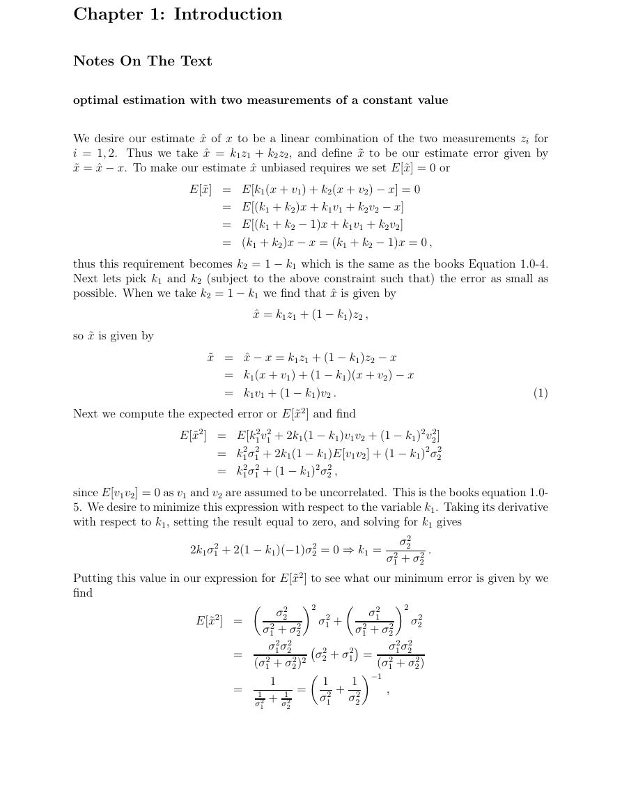
Chapter 1: Introduction Notes On The Text optimal estimation with two measurements of a constant value We desire our estimate ˆx of x to be a linear combination of the two measurements zi for i = 1, 2. Thus we take ˆx = k1z1 + k2z2, and deﬁne ˜x to be our estimate error given by ˜x = ˆx − x. To make our estimate ˆx unbiased requires we set E[˜x] = 0 or E[˜x] = E[k1(x + v1) + k2(x + v2) − x] = 0 = E[(k1 + k2)x + k1v1 + k2v2 − x] = E[(k1 + k2 − 1)x + k1v1 + k2v2] = (k1 + k2)x − x = (k1 + k2 − 1)x = 0 , thus this requirement becomes k2 = 1 − k1 which is the same as the books Equation 1.0-4. Next lets pick k1 and k2 (subject to the above constraint such that) the error as small as possible. When we take k2 = 1 − k1 we ﬁnd that ˆx is given by so ˜x is given by ˆx = k1z1 + (1 − k1)z2 , ˜x = ˆx − x = k1z1 + (1 − k1)z2 − x = k1(x + v1) + (1 − k1)(x + v2) − x = k1v1 + (1 − k1)v2 . Next we compute the expected error or E[˜x2] and ﬁnd (1) E[˜x2] = E[k2 1σ2 1σ2 = k2 = k2 1 + 2k1(1 − k1)v1v2 + (1 − k1)2v2 1v2 2] 1 + 2k1(1 − k1)E[v1v2] + (1 − k1)2σ2 1 + (1 − k1)2σ2 2 , 2 since E[v1v2] = 0 as v1 and v2 are assumed to be uncorrelated. This is the books equation 1.0- 5. We desire to minimize this expression with respect to the variable k1. Taking its derivative with respect to k1, setting the result equal to zero, and solving for k1 gives 2k1σ2 1 + 2(1 − k1)(−1)σ2 2 = 0 ⇒ k1 = σ2 2 σ2 1 + σ2 2 . Putting this value in our expression for E[˜x2] to see what our minimum error is given by we ﬁnd E[˜x2] = σ2 2 σ2 22 2)2σ2 = 1 1 + σ2 1 = 2−1 2 + σ2 1 σ2 σ2 1 + σ2 1 + σ2 σ2 1σ2 2 1 + σ2 1 + 1 σ2 2 (σ2 1 σ2 1 = = 22 1 σ2 2 σ2 1 + σ2 σ2 1σ2 2 1 + σ2 2) (σ2 ,

which is the books equation 1.06. Then our optimal estimate ˆx take the following form ˆx = σ2 2 1 + σ2 σ2 2 z1 + σ2 1 1 + σ2 σ2 2 z2 . Some special cases of the above that validate its usefulness are when each measurement contributes the same uncertainty then σ1 = σ2 and we see that ˆx = 1 2z2, or the average of the two measurements. As another special case if one measurement is exact i.e. σ1 = 0, then we have ˆx = z1 (in the same way if σ2 = 0, then ˆx = z2). 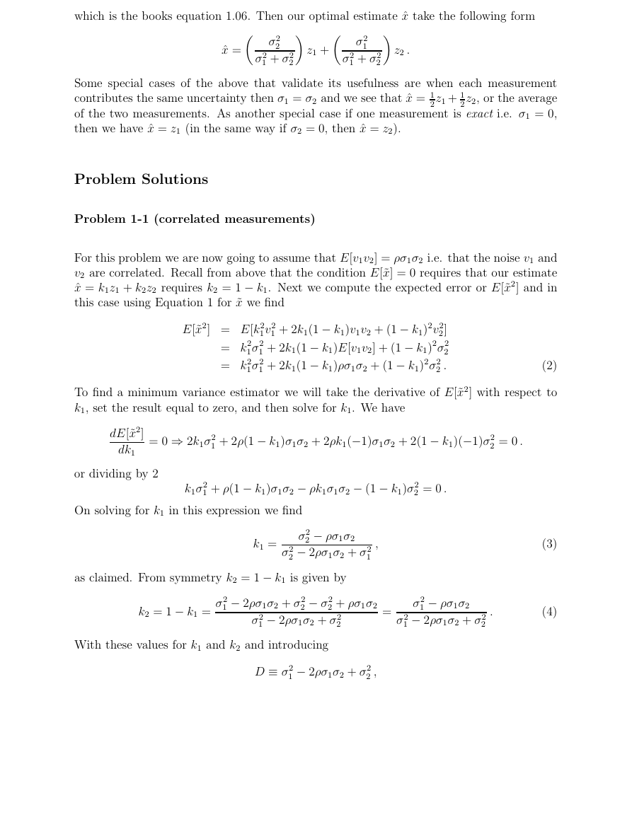2z1 + 1 Problem Solutions Problem 1-1 (correlated measurements) For this problem we are now going to assume that E[v1v2] = ρσ1σ2 i.e. that the noise v1 and v2 are correlated. Recall from above that the condition E[˜x] = 0 requires that our estimate ˆx = k1z1 + k2z2 requires k2 = 1 − k1. Next we compute the expected error or E[˜x2] and in this case using Equation 1 for ˜x we ﬁnd E[˜x2] = E[k2 1σ2 1σ2 = k2 = k2 1v2 1 + 2k1(1 − k1)v1v2 + (1 − k1)2v2 2] 1 + 2k1(1 − k1)E[v1v2] + (1 − k1)2σ2 2 1 + 2k1(1 − k1)ρσ1σ2 + (1 − k1)2σ2 2 . (2) To ﬁnd a minimum variance estimator we will take the derivative of E[˜x2] with respect to k1, set the result equal to zero, and then solve for k1. We have dE[˜x2] dk1 = 0 ⇒ 2k1σ2 1 + 2ρ(1 − k1)σ1σ2 + 2ρk1(−1)σ1σ2 + 2(1 − k1)(−1)σ2 2 = 0 . or dividing by 2 k1σ2 1 + ρ(1 − k1)σ1σ2 − ρk1σ1σ2 − (1 − k1)σ2 2 = 0 . On solving for k1 in this expression we ﬁnd k1 = σ2 2 − ρσ1σ2 σ2 2 − 2ρσ1σ2 + σ2 1 , as claimed. From symmetry k2 = 1 − k1 is given by k2 = 1 − k1 = 1 − 2ρσ1σ2 + σ2 σ2 2 − σ2 1 − 2ρσ1σ2 + σ2 σ2 2 2 + ρσ1σ2 With these values for k1 and k2 and introducing D ≡ σ2 1 − 2ρσ1σ2 + σ2 2 , (3) (4) = σ2 1 − ρσ1σ2 σ2 1 − 2ρσ1σ2 + σ2 2 .

to simplify notation the minimum mean square error given by Equation 2 becomes E[˜x2] = 1 − ρσ1σ2)σ1σ2 + (σ2 2 1 − ρσ1σ2)2σ2 = = 1 1 1σ2 1σ2 2) 1 + 2ρ(σ2 2 − ρσ3 1σ2 + ρ2σ2 D2(σ2 D2σ2 D2σ2 1σ3 2 − 2ρσ3 D2σ2 1σ4 D2 σ2 2 − ρσ1σ2)2σ2 2 − ρσ1σ2)(σ2 1σ2 2 + ρ2σ2 2 − 2ρσ1σ2σ2 1(σ4 2) 1σ2 + 2ρσ1σ2(σ2 1σ2 − ρσ1σ3 2 + ρ2σ2 2) + σ2 2(σ4 1 − 2ρσ3 1 1σ3 2 − 2ρσ3 1σ4 2 + ρ2σ4 1σ2 2 − 2ρ2σ4 2 − 2ρ2σ2 2 1σ4 1σ3 2 + ρ2σ2 2(1 − 2ρ2 + ρ2) + σ4 1(1 − ρ2) + σ1σ2(2ρ)(−1)(1 − ρ2) 2(1 − ρ2) + σ2 2 − 2ρσ1σ2 1 + σ2 2(ρ2 − 2ρ2 + 1) + σ3 1σ2 2 1σ4 2 + 2ρ3σ3 + 2ρσ3 + σ4 1σ2 1 σ2 1σ2 2 1σ2 1σ3 2 1σ3 = = σ2 1σ2 σ2 2(1 − ρ2) D2 2(1 − ρ2) 1σ2 σ2 σ2 1 − 2ρσ1σ2 + σ2 2 . = = 2(2ρ3 − 2ρ) Note that this last expression is zero when ρ = ±1. Our estimate ˆx is then given by ˆx = σ2 2 − ρσ1σ2 σ2 2 − 2ρσ1σ2 + σ2 1 z1 + σ2 1 − ρσ1σ2 σ2 1 − 2ρσ1σ2 + σ2 2 z2 . (5) As before we now consider some special cases. If ρ = +1 then the errors are totally correlated and we see that σ2 2 − σ1σ2 σ2 1 − 2σ1σ2 + σ2 2 = σ2(σ2 − σ1) (σ1 − σ2)2 = σ2 , σ2 − σ1 k1 = with k2 is given by so that ˆx is given by , k2 = 1 − k1 = −σ1 σ2 − σ1 σ2 − σ1 z2 = σ2 − σ1 z1 + −σ1 ˆx = σ2 σ2z1 − σ1z2 σ2 − σ1 . If ρ = −1 the errors are totally uncorrelated and we have σ2 σ2 2 + σ1σ2 k1 = σ2 1 + 2σ1σ2 + σ2 2 σ2 + σ1 = . with k2 is given by so that ˆx is given by k2 = 1 − k1 = σ1 σ2 − σ1 , ˆx = σ2 σ2 + σ1 z1 + σ1 σ2 + σ1 z2 = σ2z1 + σ1z2 σ2 + σ1 .

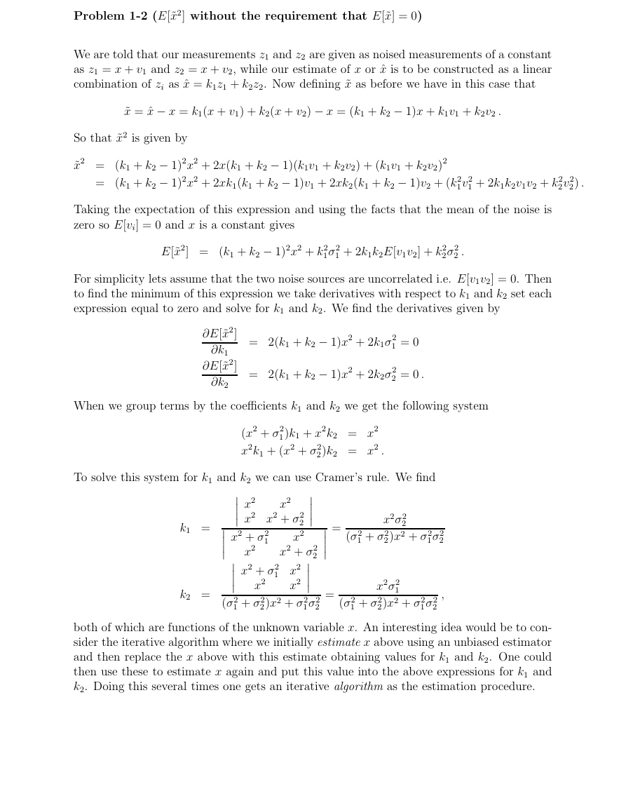
Problem 1-2 (E[˜x2] without the requirement that E[˜x] = 0) We are told that our measurements z1 and z2 are given as noised measurements of a constant as z1 = x + v1 and z2 = x + v2, while our estimate of x or ˆx is to be constructed as a linear combination of zi as ˆx = k1z1 + k2z2. Now deﬁning ˜x as before we have in this case that ˜x = ˆx − x = k1(x + v1) + k2(x + v2) − x = (k1 + k2 − 1)x + k1v1 + k2v2 . So that ˜x2 is given by ˜x2 = (k1 + k2 − 1)2x2 + 2x(k1 + k2 − 1)(k1v1 + k2v2) + (k1v1 + k2v2)2 1v2 = (k1 + k2 − 1)2x2 + 2xk1(k1 + k2 − 1)v1 + 2xk2(k1 + k2 − 1)v2 + (k2 1 + 2k1k2v1v2 + k2 2v2 2) . Taking the expectation of this expression and using the facts that the mean of the noise is zero so E[vi] = 0 and x is a constant gives E[˜x2] = (k1 + k2 − 1)2x2 + k2 1σ2 1 + 2k1k2E[v1v2] + k2 2σ2 2 . For simplicity lets assume that the two noise sources are uncorrelated i.e. E[v1v2] = 0. Then to ﬁnd the minimum of this expression we take derivatives with respect to k1 and k2 set each expression equal to zero and solve for k1 and k2. We ﬁnd the derivatives given by ∂E[˜x2] ∂k1 ∂E[˜x2] ∂k2 = 2(k1 + k2 − 1)x2 + 2k1σ2 = 2(k1 + k2 − 1)x2 + 2k2σ2 1 = 0 2 = 0 . When we group terms by the coeﬃcients k1 and k2 we get the following system (x2 + σ2 x2k1 + (x2 + σ2 1)k1 + x2k2 = x2 2)k2 = x2 . To solve this system for k1 and k2 we can use Cramer’s rule. We ﬁnd = x2σ2 2 2)x2 + σ2 1σ2 2 (σ2 1 + σ2 k1 = k2 = x2 x2 x2 x2 + σ2 x2 x2 + σ2 1 x2 x2 + σ2 x2 + σ2 1 x2 2 2 x2 1σ2 2 x2 2)x2 + σ2 1 + σ2 (σ2 = x2σ2 1 2)x2 + σ2 1σ2 2 (σ2 1 + σ2 , both of which are functions of the unknown variable x. An interesting idea would be to con- sider the iterative algorithm where we initially estimate x above using an unbiased estimator and then replace the x above with this estimate obtaining values for k1 and k2. One could then use these to estimate x again and put this value into the above expressions for k1 and k2. Doing this several times one gets an iterative algorithm as the estimation procedure.

Problem 1-3 (estimating a constant with three measurements) For this problem our three measurements are related to the unknown value of x from as z1 = x + v1, z2 = x + v2, and z3 = x + v3, and our estimate will be a linear combination of them as ˆx = k1z1 + k2z2 + k3z3. To have an unbiased estimate compute the expectation of ˜x = ˆx − x which we ﬁnd to be ˜x = ˆx − x = k1z1 + k2z2 + k3z3 − x = k1(x + v1) + k2(x + v2) + k3(x + v3) − x = (k1 + k2 + k3 − 1)x + k1v1 + k1v1 + k2v2 + k3v3 . (6) (7) To make ˆx an unbiased estimate of x we require that E[˜x] = 0. This in tern requires k1 + k2 + k3 − 1 = 0 or k3 = 1 − k1 − k2 Thus our unbiased estimate of x now takes the form ˆx = k1z1 + k2z2 + (1 − k1 − k2)z3 . We will now pick k1 and k2 such that the mean square error E[˜x2] is a minimum. With this functional form for ˆx we have using Equation 6 that ˜x2 = (k1v1 + k2v2 + k3v3)2 = k2 1v2 1 + k2 2v2 2 + k2 3v2 3 + 2k1k2v1v2 + 2k1k3v1v3 + 2k2k3v2v3 . Taking the expectation of the above expression, assuming uncorrelated measurements E[vivj] = 0 when i 6= j and recalling Equation 7 we have 2σ2 E[˜x2] = k2 1 + k2 1σ2 (8) 2 + (1 − k1 − k2)2σ2 3 . to minimize this expression we take the partial derivatives with respect to k1 and k2 and set the resulting expressions equal to zero. This gives ∂E[˜x2] ∂k1 ∂E[˜x2] ∂k2 = 2k1σ2 = 2k2σ2 1 + 2(1 − k1 − k2)(−1)σ2 2 + 2(1 − k1 − k2)(−1)σ2 3 = 0 3 = 0 . Now solving these two equations for k1 and k2 we ﬁnd k1 = k2 = σ2 2σ2 3 2 + σ2 1σ2 3 + σ2 2σ2 3 σ2 1σ2 1σ2 σ2 3 2 + σ2 1σ2 3 + σ2 2σ2 3 σ2 1σ2 = = σ32 σ1 σ32 σ2 1 1 + 1 σ22 + σ1 σ12 . + 1 + σ2

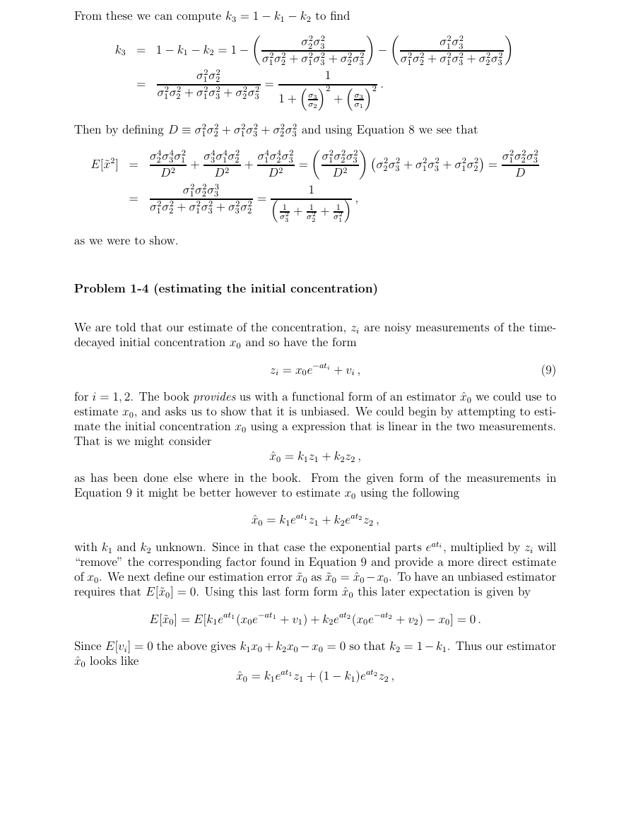
From these we can compute k3 = 1 − k1 − k2 to ﬁnd k3 = 1 − k1 − k2 = 1 − = σ2 1σ2 2 3 + σ2 1σ2 2 + σ2 2σ2 3 σ2 1σ2 = 1σ2 σ2 σ2 2σ2 3 3 + σ2 1σ2 2 + σ2 1 σ2 1σ2 3 3 + σ2 1σ2 2 + σ2 2σ2 1σ2 σ2 3 1σ2 3 + σ2 3 and using Equation 8 we see that 3 + σ2 1σ2 3 + σ2 1σ2 1σ2 2σ2 σ2 3 D 2 = 2σ2 3 − σ12 . + σ3 D2 σ2 1 , 2σ2 3 2σ2 1σ2 2σ2 3 2σ2 1 + σ3 σ22 D2 = σ2 1 + 1 σ2 2 σ2 3 1 + 1 σ2 Then by deﬁning D ≡ σ2 3σ4 σ4 1σ2 2 D2 + E[˜x2] = 2 + σ2 1σ2 2σ4 σ4 3σ2 1 D2 + 2σ3 1σ2 σ2 3 3 + σ2 1σ2 2 + σ2 1σ2 σ2 = = 3σ2 2 σ4 1σ4 as we were to show. Problem 1-4 (estimating the initial concentration) We are told that our estimate of the concentration, zi are noisy measurements of the time- decayed initial concentration x0 and so have the form zi = x0e−ati + vi , (9) for i = 1, 2. The book provides us with a functional form of an estimator ˆx0 we could use to estimate x0, and asks us to show that it is unbiased. We could begin by attempting to esti- mate the initial concentration x0 using a expression that is linear in the two measurements. That is we might consider ˆx0 = k1z1 + k2z2 , as has been done else where in the book. From the given form of the measurements in Equation 9 it might be better however to estimate x0 using the following ˆx0 = k1eat1z1 + k2eat2z2 , with k1 and k2 unknown. Since in that case the exponential parts eati, multiplied by zi will “remove” the corresponding factor found in Equation 9 and provide a more direct estimate of x0. We next deﬁne our estimation error ˜x0 as ˜x0 = ˆx0− x0. To have an unbiased estimator requires that E[˜x0] = 0. Using this last form form ˆx0 this later expectation is given by E[˜x0] = E[k1eat1(x0e−at1 + v1) + k2eat2(x0e−at2 + v2) − x0] = 0 . Since E[vi] = 0 the above gives k1x0 + k2x0 − x0 = 0 so that k2 = 1− k1. Thus our estimator ˆx0 looks like ˆx0 = k1eat1z1 + (1 − k1)eat2z2 ,

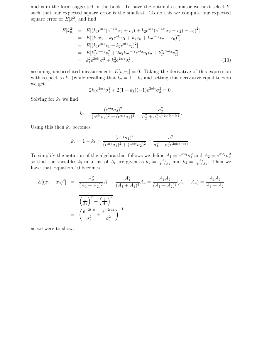
and is in the form suggested in the book. To have the optimal estimator we next select k1 such that our expected square error is the smallest. To do this we compute our expected square error or E[˜x2] and ﬁnd E[˜x2 0] = E[(k1eat1(e−at1x0 + v1) + k2eat2(e−at2x0 + v2) − x0)2] = E[(k1x0 + k1eat1v1 + k2x0 + k2eat2v2 − x0)2] = E[(k1eat1v1 + k2eat2v2)2] = E[k2 = k2 1 + 2k1k2eat1eat2v1v2 + k2 2e2at2v2 2] 1e2at1v2 2e2at2σ2 2 , 1e2at1 σ2 1 + k2 (10) assuming uncorrelated measurements E[v1v2] = 0. Taking the derivative of this expression with respect to k1 (while recalling that k2 = 1 − k1 and setting this derivative equal to zero we get 2k1e2at1σ2 1 + 2(1 − k1)(−1)e2at2 σ2 2 = 0 . Solving for k1 we ﬁnd k1 = (eat2σ2)2 (eat1σ1)2 + (eat2σ2)2 = σ2 2 1e−2a(t2−t1) . σ2 2 + σ2 Using this then k2 becomes (eat1σ1)2 k2 = 1 − k1 = σ2 1 2e2a(t2−t1) . To simplify the notation of the algebra that follows we deﬁne A1 = e2at1σ2 so that the variables ki in terms of Ai are given as k1 = A2 have that Equation 10 becomes (eat1σ1)2 + (eat2σ2)2 = 1 + σ2 σ2 A1+A2 and k2 = A1 1 and A2 = e2at2 σ2 2 . Then we A1+A2 A2 2 (A1 + A2)2 A1 + A2 1 (A1 + A2)2 A2 = A1A2 (A1 + A2)2 (A1 + A2) = A1A2 A1 + A2 E[(ˆx0 − x0)2] = = 1 A22 1 = e−2t1a σ2 1 A12 + 1 2 −1 e−2t2a σ2 + , as we were to show.

资料库

Applied+Optimal+Estimation习题答案.pdf

相关推荐

课程资源

热门标签

最新资料