Solutions Manual
for
Statistical and Adaptive Signal Processing
�
This page is intentionally left blank.
ii
�
Preface
This solutions manual provides solutions to the problems contained in the first
edition of our book STATISTICAL AND ADAPTIVE SIGNAL PROCESSING.
The solutions have been prepared and written by David Marden and ourselves. We
have attempted to provide very detailed solutions to the problems with notation
consistent with that used in the book. Where applicable, we have also given a
printout of Matlab code and figures for the problem solution.
Despite our efforts, however, you may find that some of the solutions may be less
detailed and refined than others. Inevitably through the use of this solutions man-
ual, omissions and errors will be discovered. Our goal is to continually improve
upon this manual using your comments. Periodically, we will issue changes to the
solutions manual and new problems to you upon request. In this respect, we would
appreciate any feedback including improved solutions, suggestions for new prob-
lems, corrections which can be sent to Prof. Vinay K. Ingle at vingle@ece.neu.edu
or at
Prof. Vinay K. Ingle
Department of Electrical and Computer Engineering
Northeastern University
360 Huntington Avenue
Boston, MA 02115
Thank you.
Dimitris G. Manolakis
Vinay K. Ingle
Stephen K. Kogon
iii
�
This page is intentionally left blank.
iv
�
Discrete-Time Signals and Systems
Chapter 2
2.1 Sampling frequency Fs = 100 sam/sec
(a) Continuous-time signal xc(t) = 2 cos(40πt + π /3) has frequency of 20 Hz. Hence
+ π /3
x(n) = xc (t)|t=n/Fs
= 2π
.
= 2 cos
40πn
100
which implies that ω0 = 40π
(b) Steady-state response yc,ss(t): Given that h(n) = 0.8nu(n), the frequency response function is
100
5
H (e j ω) =
1
1 − 0.8e− j ω
Since ω0 = 2π /5, the system response at ω0 is
1
H (e j ω) =
1 − 0.8e− j 2π /5
= 0.9343 e
− j 0.2517π
Hence yss(n) = 2(0.9343) cos(2πn/5 + π /3 − 0.2517π ), or
yc,ss(t) = 1. 868 6 cos(40πt + 0.585π )
(c) Any xc(t) that has the same digital frequency ω0 after sampling and the same phase shift as above will
have the same steady state response. Since Fs = 100 sam/sec, the two other frequencies are 120 and 220
Hz.
2.2 The discrete-time signal is
x(n) = A cos(ω0n) wR(n)
where wR(n) is an N-point rectangular window.
(a) The DTFT of x(n) is determined as
X (e j ω) = F [A cos(ω0n) wR(n)]
e j ω0 wR(n)
+ (A/2) F
− j ω0 wR(n)
e
Using the DTFT of wR(n) as
= (A/2) F
F [wR(n)] = N−1
n=0
− j ωn = e
e
− j ω(N−1)/2 sin(ωN /2)
sin(ω/2)
(1)
(2)
and the fact that complex exponential causes a translation in the frequency domain (1) can be written
after a fair amount of algebra and trigonometry as
X (e j ω) = XR(e j ω) + j XI(e j ω)
1
�
2
Statistical and Adaptive Signal Processing - Solution Manual
20
15
10
5
0
32−point DTFT (Real)
32−point DTFT (Imaginary)
15
10
5
0
−5
−10
−5
−4
−2
where
and
0
2
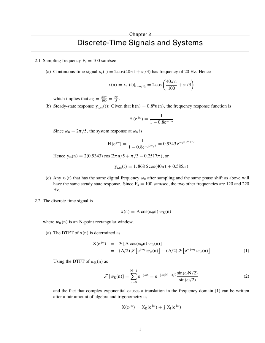
Figure 2.2bc: Real and Imaginary DTFT and DFT Plots(ω0 = π /4)
−2
0
2
4
−15
−4
4
cos[(ω − ω0)(N − 1)/2]sin[(ω − ω0)N /2]
XR(e j ω) = A
sin[(ω − ω0)/2]
2
cos[(ω + ω0)(N − 1)/2]sin{[ω − (2π − ω0)]N /2}
+ A
sin{[ω − (2π − ω0)]/2}
2
XR(e j ω) = − A
2
− A
2
sin[(ω − ω0)(N − 1)/2]sin[(ω − ω0)N /2]
sin[(ω − ω0)/2]
sin[(ω + ω0)(N − 1)/2]sin{[ω − (2π − ω0)]N /2}
sin{[ω − (2π − ω0)]/2}
(3)
(4)
(b) N = 32 and ω0 = π /4. The DTFT plots are shown in Figure 2.2bc.
(c) The DFT samples are shown in Figure 2.2bc.
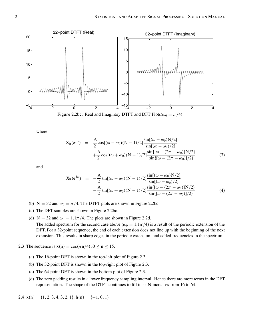
(d) N = 32 and ω0 = 1.1π /4. The plots are shown in Figure 2.2d.
The added spectrum for the second case above (ω0 = 1.1π /4) is a result of the periodic extension of the
DFT. For a 32-point sequence, the end of each extension does not line up with the beginning of the next
extension. This results in sharp edges in the periodic extension, and added frequencies in the spectrum.
2.3 The sequence is x(n) = cos(πn/4), 0 ≤ n ≤ 15.
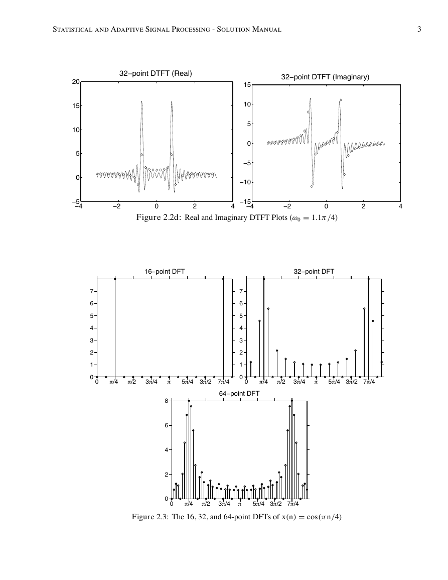
(a) The 16-point DFT is shown in the top-left plot of Figure 2.3.
(b) The 32-point DFT is shown in the top-right plot of Figure 2.3.
(c) The 64-point DFT is shown in the bottom plot of Figure 2.3.
(d) The zero padding results in a lower frequency sampling interval. Hence there are more terms in the DFT
representation. The shape of the DTFT continues to fill in as N increases from 16 to 64.
2.4 x(n) = {1, 2, 3, 4, 3, 2, 1}; h(n) = {−1, 0, 1}
�
Statistical and Adaptive Signal Processing - Solution Manual
3
20
15
10
5
0
32−point DTFT (Real)
32−point DTFT (Imaginary)
15
10
5
0
−5
−10
−5
−4
−2
0
2
Figure 2.2d: Real and Imaginary DTFT Plots (ω0 = 1.1π /4)
−15
−4
4
−2
0
2
4
16−point DFT
32−point DFT
7
6
5
4
3
2
1
0
0
π/4
π/2
3π/4
π
7
6
5
4
3
2
1
0
5π/4 3π/2 7π/4
0
64−point DFT
π/4
π/2 3π/4
π
5π/4 3π/2 7π/4
8
6
4
2
0
π/4
π/2 3π/4 π
5π/4 3π/2 7π/4
Figure 2.3: The 16, 32, and 64-point DFTs of x(n) = cos(π n/4)
0
�
4
Statistical and Adaptive Signal Processing - Solution Manual
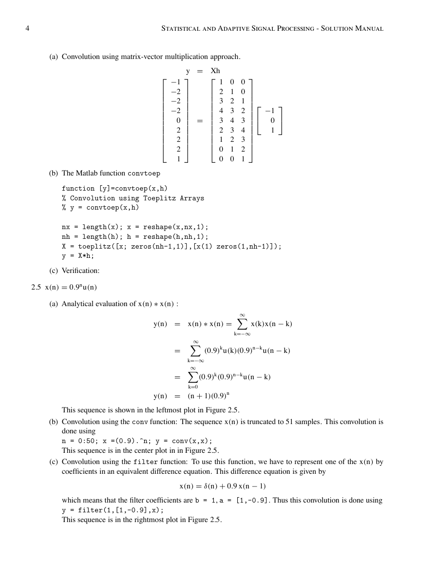
(a) Convolution using matrix-vector multiplication approach.
y = Xh
−1−2−2−2
0
2
2
2
1
=
−1
0
1
1 0 0
2 1 0
3 2 1
4 3 2
3 4 3
2 3 4
1 2 3
0 1 2
0 0 1
(b) The Matlab function convtoep
function [y]=convtoep(x,h)
% Convolution using Toeplitz Arrays
% y = convtoep(x,h)
nx = length(x); x = reshape(x,nx,1);
nh = length(h); h = reshape(h,nh,1);
X = toeplitz([x; zeros(nh-1,1)],[x(1) zeros(1,nh-1)]);
y = X*h;
(c) Verification:
2.5 x(n) = 0.9nu(n)
(a) Analytical evaluation of x(n) ∗ x(n) :
y(n) = x(n) ∗ x(n) =
∞
k=−∞
x(k)x(n − k)
(0.9)ku(k)(0.9)n−ku(n − k)
∞
∞
k=−∞
=
=
(0.9)k(0.9)n−ku(n − k)
k=0
y(n) = (n + 1)(0.9)n
This sequence is shown in the leftmost plot in Figure 2.5.
(b) Convolution using the conv function: The sequence x(n) is truncated to 51 samples. This convolution is
done using
n = 0:50; x =(0.9).^n; y = conv(x,x);
This sequence is in the center plot in in Figure 2.5.
(c) Convolution using the filter function: To use this function, we have to represent one of the x(n) by
coefficients in an equivalent difference equation. This difference equation is given by
x(n) = δ(n) + 0.9 x(n − 1)
which means that the filter coefficients are b = 1, a = [1,-0.9]. Thus this convolution is done using
y = filter(1,[1,-0.9],x);
This sequence is in the rightmost plot in Figure 2.5.
�





 2023年江西萍乡中考道德与法治真题及答案.doc
 2012年重庆南川中考生物真题及答案.doc
 2013年江西师范大学地理学综合及文艺理论基础考研真题.doc
 2020年四川甘孜小升初语文真题及答案I卷.doc
 2020年注册岩土工程师专业基础考试真题及答案.doc
 2023-2024学年福建省厦门市九年级上学期数学月考试题及答案.doc
 2021-2022学年辽宁省沈阳市大东区九年级上学期语文期末试题及答案.doc
 2022-2023学年北京东城区初三第一学期物理期末试卷及答案.doc
 2018上半年江西教师资格初中地理学科知识与教学能力真题及答案.doc
 2012年河北国家公务员申论考试真题及答案-省级.doc
 2020-2021学年江苏省扬州市江都区邵樊片九年级上学期数学第一次质量检测试题及答案.doc
 2022下半年黑龙江教师资格证中学综合素质真题及答案.doc