OpenSYMORO: An open-source software package for
Symbolic Modelling of Robots
Wisama Khalil, Aravindkumar Vijayalingam, Bogdan Khomutenko, Izzatbek Mukhanov,
Philippe Lemoine, Ga¨el Ecorchard
´Ecole Centrale de Nantes, IRCCyN UMR CNRS 6597
1 rue de la No¨e, BP 92101, 44321 Nantes Cedex 3, France
Abstract— This paper presents OpenSYMORO, an open-
source software package for symbolic modelling of robots. This
software package is based on previous work detailed in [1].
However, the package in [1] was developed using Wolfram
Mathematica and hence required Mathematica license for
use. OpenSYMORO is mainly developed using the Python
programming language and the source code will be publicly
available. The new version provides support to model robots
with flexible joints, floating base and wheeled mobile robots.
This is in addition to supporting serial, tree structure and
closed-loop robots. A visualisation tool to view the structure
of the robot is also included.
the robot and the output of inverse geometric models can be
obtained in a format that is compatible with Matlab and
Python such that the generated equations can be directly
used by these systems.
In the next section of this paper, the architecture and the
different components of the software package are discussed.
A short presentation on how to define a robot in SYMORO
follows. Thereafter, the algorithms used to model robots with
flexible joints, floating base and wheeled mobile robots are
detailed.
I. INTRODUCTION
II. SOFTWARE PACKAGE DESCRIPTION
Symbolic modelling of robots is essential for analysis and
design of robots and their controllers. Also symbolic mod-
elling results in lower execution time and is more convenient
for analysis. For instance, solution to the inverse geometric
problem can be obtained by the use of differential model to
compute an iterative numerical solution [2]. However, this
results in long execution time and may not be practical. On
the other hand the solution for the same inverse geometric
problem can be obtained using closed-form symbolic models
that can deliver all the possible solutions with a lower and
predictable computation time.
The purpose of OpenSYMORO (henceforth referred to as
SYMORO) software package is to compute the symbolic
models of a robot that are needed for design, identification,
control and simulation. Previously, such a package was
presented in [1]. However, the package in [1] was developed
using Wolfram Mathematica1 and hence required Mathe-
matica license for use. The new version of the package is
developed using Python programming language and other
third-party libraries – SymPy2 and NumPy3 that are available
for use without any licensing requirements. As a result, the
SYMORO package is available as an open-source project and
the source code will be publicly available. Consequently the
robotics community over the world can use this package and
can take part in the development of new modules.
Additionally, the new version of SYMORO software pack-
age provides support to model robots with flexible joints,
floating base and wheeled mobile robots. The new version
also provides a visualisation tool to view the structure of
1http://www.wolfram.com/mathematica/
2http://www.sympy.org/
3http://www.numpy.org/
The SYMORO software package is made up of five
different sub-packages. These sub-packages are –
symoroutils, pysymoro, symoroui, symoroviz
and symorooptim. These sub-packages may depend on
another sub-package/s.
A. symoroutils
The symoroutils package contains the utility modules
for mathematical functions and file handling. The file han-
dling modules include the functions to perform parsing of
files that are used to load robot data into the environment.
B. pysymoro
The algorithms that are used to generate the different
models that can be obtained using SYMORO are contained
in this package. The data structures that are used to store
the robot data and models are also present in this package.
This package in turn makes use of SymPy and NumPy to
perform the symbolic and numeric computations.
C. symoroui
The symoroui package provides the graphical user inter-
face for the SYMORO software. The user interface created
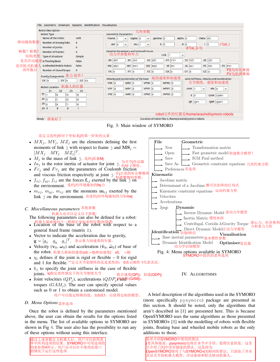
using wxPython4 is shown in Fig 3. This package permits
to define the parameters that are needed in the calculation of
different models. This interface is also used to execute any
desired model.
4http://www.wxpython.org/
�
D. symorooptim
The purpose of this package is to generate optimised
models in symbolic form. These optimised models reduce
the total number of operations (addition and multiplication)
required to compute the respective models by the use of
intermediate variables. The output of the optimised models
can be obtained in a format
is compatible with C,
Python, Matlab, such that the generated model can be
directly used by these systems.
that
• γj , bj , αj , dj , θj and rj to define a frame j with respect
to its antecedent frame a(j). The terms γj and bj are
zero in a serial robot. The joint variable qj is either θj
or rj depending on the joint type.
• σj defines the joint type – 0 for revolute, 1 for prismatic
and 2 for a frame that has a constant relationship with
it’s antecedent. For revolute and prismatic joints, ¯σj =
1 − σj .
• µj indicates if a joint is active (actuated) or passive
(non-actuated) – 1 for active and 0 for passive. For open-
loop robots – serial and tree structure all the joints are
supposed actuated.
• a(j) to indicate the antecedent frame. Here “0” indicates
the base.
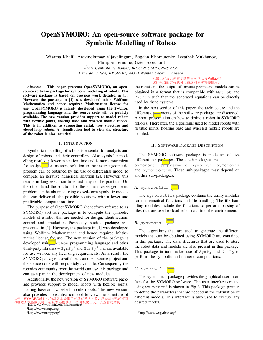
Fig. 1: Representation of Staubli RX-90 robot
E. symoroviz
This package developed using the Python port of OpenGL
helps with visualisation of robots. As can be seen from Fig
1, in addition to drawing the joints of a robot this package
also draws the frames corresponding to each joint according
to the modified Denavit and Hartenberg method as proposed
by Khalil and Kleinfinger [3]. This permits to verify if the
user has properly defined the different frames attached to
each of the links.
III. ROBOT DESCRIPTION AND MENU OPTIONS
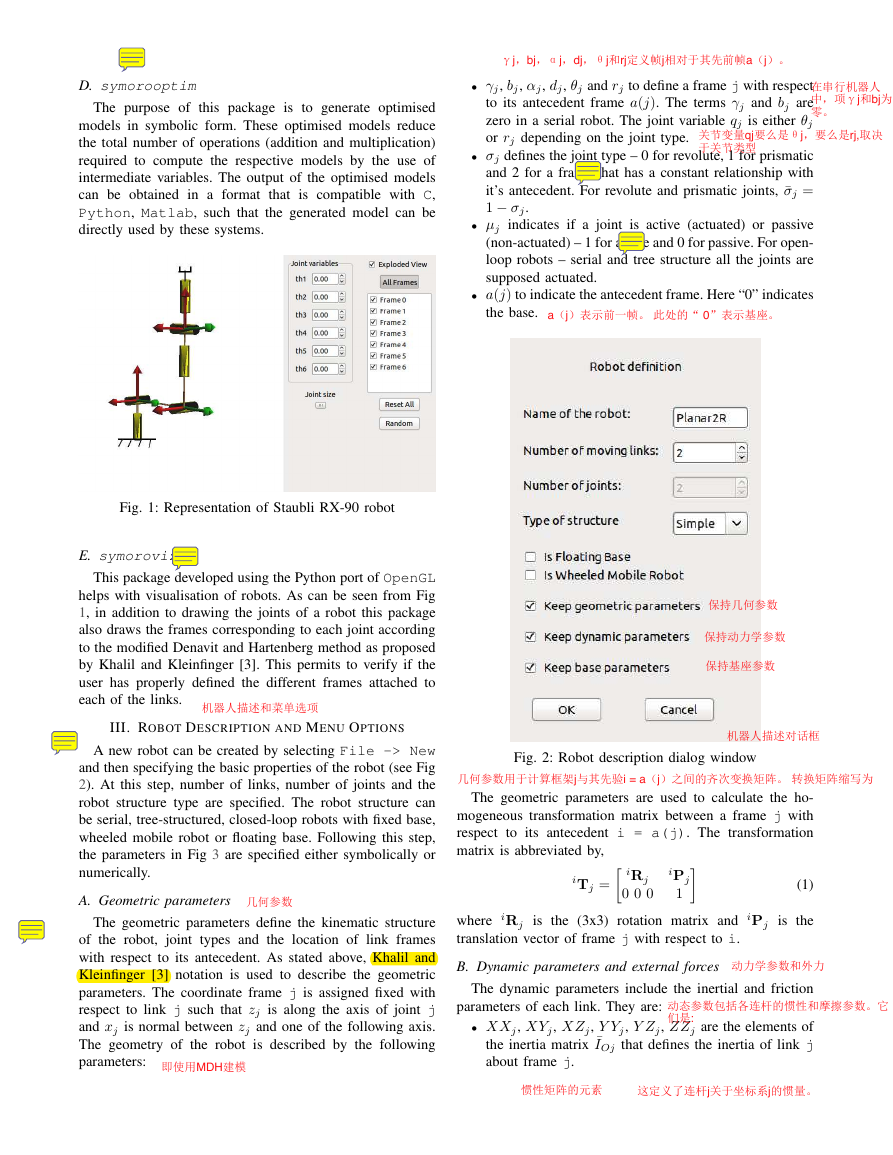
A new robot can be created by selecting File -> New
and then specifying the basic properties of the robot (see Fig
2). At this step, number of links, number of joints and the
robot structure type are specified. The robot structure can
be serial, tree-structured, closed-loop robots with fixed base,
wheeled mobile robot or floating base. Following this step,
the parameters in Fig 3 are specified either symbolically or
numerically.
A. Geometric parameters
Fig. 2: Robot description dialog window
The geometric parameters are used to calculate the ho-
mogeneous transformation matrix between a frame j with
respect to its antecedent i = a(j). The transformation
matrix is abbreviated by,
iTj = iRj
0 0 0
(1)
iPj
1
The geometric parameters define the kinematic structure
of the robot, joint types and the location of link frames
with respect to its antecedent. As stated above, Khalil and
Kleinfinger [3] notation is used to describe the geometric
parameters. The coordinate frame j is assigned fixed with
respect to link j such that zj is along the axis of joint j
and xj is normal between zj and one of the following axis.
The geometry of the robot is described by the following
parameters:
where iRj
translation vector of frame j with respect to i.
is the (3x3) rotation matrix and iPj
is the
B. Dynamic parameters and external forces
The dynamic parameters include the inertial and friction
parameters of each link. They are:
• XXj , XYj , XZj , Y Yj , Y Zj , ZZj are the elements of
the inertia matrix ¯IOj that defines the inertia of link j
about frame j.
�
Fig. 3: Main window of SYMORO
• M Xj , M Yj , M Zj are the elements defining the first
moments of link j with respect to frame j and MSj =
[M Xj M Yj M Zj]T .
• Mj is the mass of link j.
• Iaj is the rotor inertia of actuator for joint j.
• F cj and F vj are the parameters of Coulomb friction
File
Geometric
New
Open
Save
Save As
Preferences
Transformation matrix
Fast geometric model
IGM Paul method
Geometric constraint equations
and viscous friction respectively at joint j.
Kinematic
• fxj , fyj , fzj are the forces fej exerted by the link j on
the environment.
• mxj , myj , mzj are the moments mej exerted by the
link j on the environment.
C. Miscellaneous parameters
The following parameters can also be defined for a robot:
• Location of the base of the robot with respect to a
general fixed frame (matrix Z).
• Vector to indicate the acceleration due to gravity,
g = [gx
gy
gz]T .
• Velocity (v0, ω0) and acceleration ( ˙v0, ˙ω0) of base of
Jacobian matrix
Determinant of a Jacobian
Kinematic constraint equations
Velocities
Accelerations
Jpqp
Dynamic
Inverse Dynamic Model
Inertia Matrix
Centrifugal, Coriolis &Gravity Torque
Direct Dynamic Model
Identification
Base inertial parameters
Dynamic Identification Model
Visualisation
Optimiser
the robot.
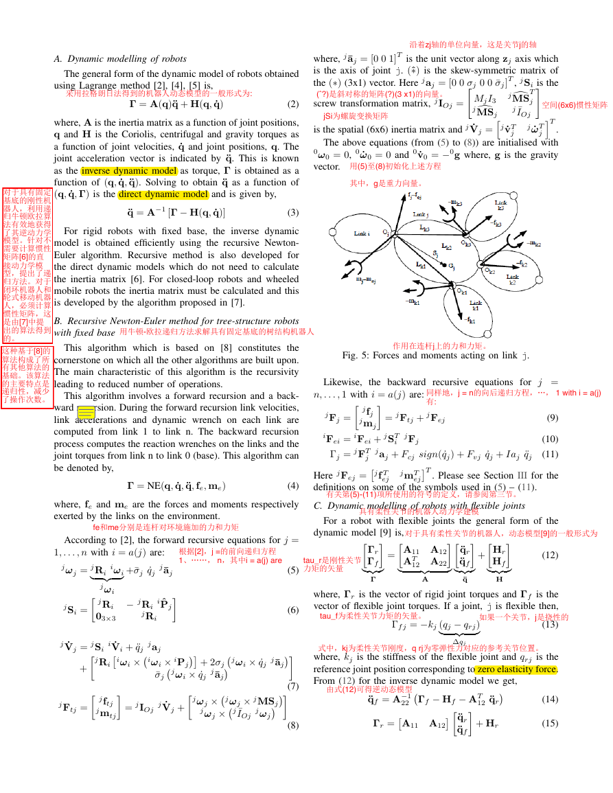
Fig. 4: Menu options available in SYMORO
• ηj defines if the joint is rigid or flexible – 0 for rigid
and 1 for flexible.
• kj to specify the joint stiffness in the case of flexible
joints.
• Joint velocities (QPj ), accelerations (QDPj ) and
torques (GAMj ). The user can specify special values
such as 0 or 1 to obtain a customised model.
D. Menu Options
Once the robot is defined by the parameters mentioned
above, the user can obtain the results for the options listed
in the menu. The list of available options in SYMORO are
shown in Fig 4. The user also has the possibility to run any
of these options without using this interface.
IV. ALGORITHMS
A brief description of the algorithms used in the SYMORO
(more specifically pysymoro) package are presented in
this section. It should be noted, only the algorithms that
aren’t described in [1] are presented here. This is because
OpenSYMORO uses the same algorithms as those presented
in SYMORO+ [1] with the modelling of robots with flexible
joints, floating base and wheeled mobile robots as the only
additions to those.
�
A. Dynamic modelling of robots
The general form of the dynamic model of robots obtained
using Lagrange method [2], [4], [5] is,
Γ = A(q)¨q + H(q, ˙q)
(2)
where, A is the inertia matrix as a function of joint positions,
q and H is the Coriolis, centrifugal and gravity torques as
a function of joint velocities, ˙q and joint positions, q. The
joint acceleration vector is indicated by ¨q. This is known
as the inverse dynamic model as torque, Γ is obtained as a
function of (q, ˙q, ¨q). Solving to obtain ¨q as a function of
(q, ˙q, Γ) is the direct dynamic model and is given by,
¨q = A−1 [Γ − H(q, ˙q)]
(3)
For rigid robots with fixed base,
the inverse dynamic
model is obtained efficiently using the recursive Newton-
Euler algorithm. Recursive method is also developed for
the direct dynamic models which do not need to calculate
the inertia matrix [6]. For closed-loop robots and wheeled
mobile robots the inertia matrix must be calculated and this
is developed by the algorithm proposed in [7].
B. Recursive Newton-Euler method for tree-structure robots
with fixed base
This algorithm which is based on [8] constitutes the
cornerstone on which all the other algorithms are built upon.
The main characteristic of this algorithm is the recursivity
leading to reduced number of operations.
This algorithm involves a forward recursion and a back-
ward recursion. During the forward recursion link velocities,
link accelerations and dynamic wrench on each link are
computed from link 1 to link n. The backward recursion
process computes the reaction wrenches on the links and the
joint torques from link n to link 0 (base). This algorithm can
be denoted by,
Γ = NE(q, ˙q, ¨q, fe, me)
(4)
where, j¯aj = [0 0 1]T is the unit vector along zj axis which
is the axis of joint j. (ˆ∗) is the skew-symmetric matrix of
the (∗) (3x1) vector. Here j aj = [0 0 σj 0 0 ¯σj]T , j Si is the
screw transformation matrix, j IOj =" MjI3
j ¯IOj #
jdMS
jdMSj
jiT
is the spatial (6x6) inertia matrix and j ˙Vj =hj ˙vT
.
The above equations (from (5) to (8)) are initialised with
0ω0 = 0, 0 ˙ω0 = 0 and 0 ˙v0 = −0g where, g is the gravity
vector.
j ˙ωT
T
j
j
Fig. 5: Forces and moments acting on link j.
Likewise,
the backward recursive equations for j =
n, . . . , 1 with i = a(j) are:
j Fj = j fj
jmj = j Ftj + j Fej
iFei = iFei + j ST
i
j Fj
Γj = j FT
j
j aj + Fcj sign( ˙qj) + Fvj ˙qj + Iaj ¨qj
(9)
(10)
(11)
Here j Fej =j f T
ej
jmT
ejT
definitions on some of the symbols used in (5) – (11).
. Please see Section III for the
where, fe and me are the forces and moments respectively
exerted by the links on the environment.
C. Dynamic modelling of robots with flexible joints
For a robot with flexible joints the general form of the
According to [2], the forward recursive equations for j =
1, . . . , n with i = a(j) are:
jωj = j Ri
iωi
+¯σj ˙qj
j¯aj
| {z }
jωi
j Si = j Ri − j Ri
03×3
j Ri
i ˆPj
(5)
(6)
j ˙Vj = j Si
i ˙Vi + ¨qj
j aj
j¯aj
+j Riiωi ×iωi × iPj + 2σjjωi × ˙qj
j¯aj
¯σjjωi × ˙qj
j ˙Vj +jωj ×jωj × jMSj
jmtj = j IOj
jωj
jωj ×j ¯IOj
j Ftj = j ftj
(7)
(8)
dynamic model [9] is,
Γf
Γr
|{z}Γ
AT
12 A22
=A11 A12
|
}
{z
A
¨qr
¨qf
|{z}¨q
+Hr
Hf
|{z}H
(12)
where, Γr is the vector of rigid joint torques and Γf is the
vector of flexible joint torques. If a joint, j is flexible then,
Γf j = −kj (qj − qrj)
(13)
|
∆qj
{z
}
where, kj is the stiffness of the flexible joint and qrj is the
reference joint position corresponding to zero elasticity force.
From (12) for the inverse dynamic model we get,
¨qf = A−1
22 Γf − Hf − AT
12 ¨qr
¨qf + Hr
Γr =A11 A12¨qr
(14)
(15)
�
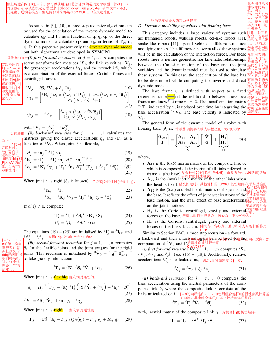
As stated in [9], [10], a three step recursive algorithm can
be used for the calculation of the inverse dynamic model to
calculate ¨qf and Γr as a function of q, ˙q, ¨qr or the direct
dynamic model to calculate ¨qf and ¨qr in terms of Γr, q,
˙q. In this paper we present only the inverse dynamic model
but both algorithms are developed in SYMORO.
(i) first forward recursion for j = 1, . . . , n computes the
screw transformation matrices j Si, the link velocities j Vj ,
the gyroscopic accelerations jγ j and the wrench jβj which
is a combination of the external forces, Coriolis forces and
centrifugal forces.
(16)
j Vj = j Si
iVi + ˙qj
j aj
j¯aj
jγ j =j Riiωi ×iωi × iPj + 2σjjωi × ˙qj
j¯aj
jβj = − j Fej −jωj ×jωj × jMSj
jωj
with j Vj =j vT
¯σjjωi × ˙qj
jωj ×j ¯IOj
jT
(ii) backward recursion for j = n, . . . , 1 calculates the
matrices giving the elastic accelerations ¨qj and j Fj as a
function of i ˙Vi. When joint j is flexible,
jωT
(17)
(18)
.
j
Hj = j aj
j Kj = j I∗
jαj = j Kj
T j I∗
j
j − j I∗
j
j aj
j aj H −1
j
j aj
T j I∗
j
jγ j + j Ij
∗ j aj H −1
j
(19)
(20)
j − jβ∗
j
(21)
T jβ∗
Γf j + j aj
When joint j is rigid (¨qj is known),
j Kj = j I∗
j
jαj = j Kj
jγ j + j Ij
∗ j aj ¨qj − jβ∗
j
If a(j) 6= 0, compute:
iI∗
iβ∗
i = iI∗
i = iβ∗
i + j Si
i − j Si
T j Kj
T jαj
j Si
(22)
(23)
(24)
(25)
The equations (19) – (25) are initialised by j I∗
jβ∗
j = jβj .
(iii) second forward recursion for j = 1, . . . , n computes
¨qj for the flexible joints and the joint torques for the rigid
joints. This recursion is initialised by 0 ˙V0 = [0gT 0T
3×1]T
to take gravity into account.
j = j IOj and
D. Dynamic modelling of robots with floating base
This category includes a large variety of systems such
as: humanoid robots, walking robots, eel-like robots [11],
snake-like robots [11], spatial vehicles, offshore structures
and flying robots. The difference between all of these systems
will be in the calculation of the interaction forces. For these
robots there is neither geometric nor kinematic relationships
between the Cartesian motion of the base and the joint
variables and the dynamic model must be used to simulate
these systems. In this case, the acceleration of the base has
to be determined while computing the inverse and direct
dynamic models.
The base frame 0 is defined with respect
to a fixed
reference frame W and the relationship between these two
frames are known at time t = 0. The transformation matrix
W T0 indicated by Z, is updated over time by integrating the
base acceleration W ˙Vb. The base velocity is indicated by
Vb.
The general form of the dynamic model of a robot with
floating base [9] is,
12 A22
Γ =A11 A12
06×1
}
{z
|
AT
A
H2
¨q +H1
0 ˙V0
|{z}H
(30)
where,
• A11 is the (6x6) inertia matrix of the composite link 0,
which is composed of the inertia of all links referred to
frame 0 (the base).
• A22 is the (nxn) inertia matrix of the other links when
the head is fixed.
• A12 is the (6xn) coupled inertia matrix of the joints and
the base. It reflects the effect of joint accelerations of the
base motion, and the dual effect of base accelerations
on the joint motions.
• H1 is the Coriolis, centrifugal, gravity and external
forces on the base.
• H2 is the Coriolis, centrifugal, gravity and external
forces on the links 1, . . . , n.
Similar to Section IV-C, a three step recursion - a forward,
a backward and then a forward again can be used for the
computation of 0 ˙V0 and Γ.
(i) first forward recursion for j = 1, . . . , n computes j Si,
j Vj , jγ j and jβj (see (16) – (18)). Additionally, relative
accelerations jζj is calculated as,
j Fj = j Kj
j Si
i ˙Vi + jαj
(26)
jζj = jγ j + ¨qj
j aj
(31)
When joint j is flexible,
¨qj = H −1
j
hΓf j − j aT
j
j I∗
jj Si
i ˙Vi + jγ j + j aj
T jβ∗
ji(27)
j ˙Vj = j Si
i ˙Vi + j aj ¨qj + jγ j
(28)
When joint j is rigid,
Γj = j FT
j
j aj + Fcj sign( ˙qj) + Fvj ˙qj + Iaj ¨qj
(29)
(ii) backward recursion for j = n, . . . , 0 computes the
base acceleration using the inertial parameters of the com-
posite link 0, where the composite link j consists of the
links articulated on it.
j Fj = j Ic
j
j ˙Vj − jβc
j
with, inertial matrix of the composite link j,
iIc
i = iIc
i + j ST
i
j Ic
j
j Si
(32)
(33)
�
and
iβc
i = iβc
i + j ST
i
jβc
j − j ST
i
j Ic
j
jζj
(34)
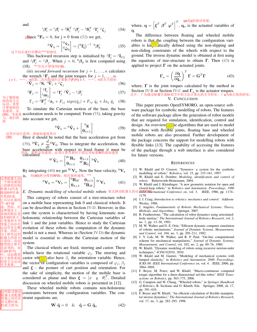
Since 0F0 = 0, for j = 0 from (32) we get,
0 ˙V0 = 0 ˙v0
0 ˙ω0 =0Ic
0−1 0βc
0
This backward recursion step is initialised by j Ic
j = j IOj
j = jβj . When j = 0, 0β0 is first computed using
and jβc
(18).
(iii) second forward recursion for j = 1, . . . , n calculates
the wrench j Fj and the joint torques for j = 1, . . . , n.
j ˙Vj = j Si
i ˙Vi + jζj
j Fj = j fj
jmj = j Ic
j
j ˙Vj − jβc
j
Γj = j FT
j
j aj + Fcj sign( ˙qj) + Fvj ˙qj + Iaj ¨qj
To simulate the Cartesian motion of the base, the base
acceleration needs to be computed. From (35), taking gravity
into account we get,
0 ˙Vb = 0 ˙V0 + 0g
03×1
Here it should be noted that the base acceleration got from
(39), 0 ˙Vb 6=
0V0. Thus to integrate the acceleration, the
base acceleration with respect to fixed frame W must be
calculated.
d
dt
By integrating (40) we get W Vb. Now the base velocity, 0Vb
is,
03×3
W R0 0 ˙Vb
W ˙Vb =W R0 03×3
0V0 = 0Vb =0RW 03×3
0RW W Vb
03×3
E. Dynamic modelling of wheeled mobile robots
This category of robots consist of a tree-structure robot
on a mobile base representing link 0 and classical wheels. It
can be described as shown in Section IV-D. However, in this
case the system is characterised by having kinematic non-
holonomic relationship between the Cartesian variables of
link 0 and the joint variables. Hence to study the Cartesian
evolution of these robots the computation of the dynamic
model is not a must. Whereas in (Section IV-D) the dynamic
model is essential to obtain the Cartesian motion of the
system.
The classical wheels are fixed, steering and castor. These
wheels have the rotational variable ϕj . The steering and
castor wheels also have βj the orientation variable. Hence,
the vector of configuration variables is composed of ϕj , βj
and ξ - the posture of cart position and orientation. For
the sake of simplicity, the motion of the mobile base is
θ]T . Detailed
considered as planar and thus ξ = [x y
discussion on wheeled mobile robots is presented in [12].
These wheeled mobile robots contains non-holonomic
constraints between the configuration variables. The con-
straint equations are,
W ˙q = 0 & ˙q = G ˙qa
(42)
(40)
REFERENCES
(35)
(36)
(37)
(38)
(39)
(41)
where, q =hξT βT ϕTiT
q.
, qa is the actuated variables of
The difference between floating and wheeled mobile
robots is that the coupling between the configuration vari-
ables is kinematically defined using the non-slipping and
non-sliding constraints of the wheels with respect to the
ground. The inverse dynamic model is obtained at first using
the equations of tree-structure to obtain Γ. Then (43) is
applied to project Γ on the actuated joints.
Γa = ∂ ˙q
∂ ˙qaT
Γ = GT Γ
(43)
where, Γ is the joint torques calculated by the method in
Section IV-B or Section IV-C and Γa is the actuator torques.
V. CONCLUSION
This paper presents OpenSYMORO, an open-source soft-
ware package for symbolic modelling of robots. The features
of the software package allow the generation of robot models
that are required for simulation, identification, control and
design. An overview of the algorithms that are used to model
the robots with flexible joints, floating base and wheeled
mobile robots are also presented. Further development of
the package concerns the support for modelling robots with
flexible links [13]. The capability of accessing the features
of the package through a web interface is also considered
for future versions.
[1] W. Khalil and D. Creusot, “Symoro+: a system for the symbolic
modelling of robots,” Robotica, vol. 15, pp. 153–161, 1997.
[2] W. Khalil and E. Dombre, Modeling, identification and control of
robots. Butterworth-Heinemann, 2004.
[3] W. Khalil and J. Kleinfinger, “A new geometric notation for open and
closed-loop robots,” in Robotics and Automation. Proceedings. 1986
IEEE International Conference on, vol. 3.
IEEE, 1986, pp. 1174–
1179.
[4] J. J. Craig, Introduction to robotics: mechanics and control. Addison-
Wesley, 1986.
[5] J. Angeles, Fundamentals of Robotic Mechanical Systems: Theory,
Methods, and Algorithms. Springer, 2007.
[6] R. Featherstone, “The calculation of robot dynamics using articulated-
body inertias,” The International Journal of Robotics Research, vol. 2,
no. 1, pp. 13–30, 1983.
[7] M. W. Walker and D. E. Orin, “Efficient dynamic computer simulation
of robotic mechanisms,” Journal of Dynamic Systems, Measurement,
and Control, vol. 104, no. 3, pp. 205–211, 1982.
[8] J. Y. Luh, M. W. Walker, and R. P. Paul, “On-line computational
scheme for mechanical manipulators,” Journal of Dynamic Systems,
Measurement, and Control, vol. 102, no. 2, pp. 69–76, 1980.
[9] W. Khalil, “Dynamic modeling of robots using recursive newton-euler
techniques,” ICINCO2010, 2010.
[10] W. Khalil and M. Gautier, “Modeling of mechanical systems with
lumped elasticity,” in Robotics and Automation, 2000. Proceedings.
ICRA’00. IEEE International Conference on, vol. 4.
IEEE, 2000, pp.
3964–3969.
[11] F. Boyer, M. Porez, and W. Khalil, “Macro-continuous computed
torque algorithm for a three-dimensional eel-like robot,” IEEE Trans-
actions on Robotics, pp. 563–775, 2006.
[12] G. Campion and W. Chung, “Wheeled robots,” in Springer Handbook
of Robotics, B. Siciliano and O. Khatib, Eds. Springer, 2008, ch. 17,
pp. 391–410.
[13] F. Boyer and W. Khalil, “An efficient calculation of flexible manipula-
tor inverse dynamics,” The International Journal of Robotics Research,
vol. 17, no. 3, pp. 282–293, 1998.
�


 2023年江西萍乡中考道德与法治真题及答案.doc
 2012年重庆南川中考生物真题及答案.doc
 2013年江西师范大学地理学综合及文艺理论基础考研真题.doc
 2020年四川甘孜小升初语文真题及答案I卷.doc
 2020年注册岩土工程师专业基础考试真题及答案.doc
 2023-2024学年福建省厦门市九年级上学期数学月考试题及答案.doc
 2021-2022学年辽宁省沈阳市大东区九年级上学期语文期末试题及答案.doc
 2022-2023学年北京东城区初三第一学期物理期末试卷及答案.doc
 2018上半年江西教师资格初中地理学科知识与教学能力真题及答案.doc
 2012年河北国家公务员申论考试真题及答案-省级.doc
 2020-2021学年江苏省扬州市江都区邵樊片九年级上学期数学第一次质量检测试题及答案.doc
 2022下半年黑龙江教师资格证中学综合素质真题及答案.doc