A Comprehensive Survey on Graph Neural Network（2019）.pdf

发布时间：2022-05-31 发布人：admin 分类：说明书资料大小：1.81M 资料格式：pdf 举报版权申诉

yyl424525-11594336-4744300845377866416.pdf-第1页.png

第1页 / 共22页

yyl424525-11594336-4744300845377866416.pdf-第2页.png

第2页 / 共22页

yyl424525-11594336-4744300845377866416.pdf-第3页.png

第3页 / 共22页

yyl424525-11594336-4744300845377866416.pdf-第4页.png

第4页 / 共22页

yyl424525-11594336-4744300845377866416.pdf-第5页.png

第5页 / 共22页

yyl424525-11594336-4744300845377866416.pdf-第6页.png

第6页 / 共22页

yyl424525-11594336-4744300845377866416.pdf-第7页.png

第7页 / 共22页

yyl424525-11594336-4744300845377866416.pdf-第8页.png

第8页 / 共22页

1 Introduction

2 Definition

3 Categorization and Frameworks

3.1 Taxonomy of GNNs

3.2 Frameworks

4 Graph Convolution Networks

4.1 Spectral-based Graph Convolutional Networks

4.1.1 Backgrounds

4.1.2 Methods of Spectral-based GCNs

4.1.3 Summary

4.2 Spatial-based Graph Convolutional Networks

4.2.1 Recurrent-based Spatial GCNs

4.2.2 Composition Based Spatial GCNs

4.2.3 Miscellaneous Variants of Spatial GCNs

4.2.4 Summary

4.3 Graph Pooling Modules

4.4 Comparison Between Spectral and Spatial Models

5 Beyond Graph Convolutional Networks

5.1 Graph Attention Networks

5.1.1 Methods of Graph Attention Networks

5.1.2 Summary

5.2 Graph Auto-encoders

5.2.1 GCN Based Auto-encoders

5.2.2 Miscellaneous Variants of Graph Auto-encoders

5.2.3 Summary

5.3 Graph Generative Networks

5.3.1 GCN Based Graph Generative Networks

5.3.2 Miscellaneous Graph Generative Networks

5.3.3 Summary

5.4 Graph Spatial-Temporal Networks

5.4.1 GCN Based Graph Spatial-Temporal Networks

5.4.2 Miscellaneous Variants

5.4.3 Summary

6 Applications

6.1 Datasets

6.2 Benchmarks & Open-source Implementations

6.3 Practical Applications

7 Future Directions

8 Conclusion

References

9 1 0 2 r a M 0 1 ] G L . s c [ 2 v 6 9 5 0 0 . 1 0 9 1 : v i X r a JOURNAL OF LATEX CLASS FILES, VOL. X, NO. X, DECEMBER 2018 1 A Comprehensive Survey on Graph Neural Networks Zonghan Wu, Shirui Pan, Member, IEEE, Fengwen Chen, Guodong Long, Chengqi Zhang, Senior Member, IEEE, Philip S. Yu, Fellow, IEEE Abstract—Deep learning has revolutionized many machine learning tasks in recent years, ranging from image classiﬁcation and video processing to speech recognition and natural language understanding. The data in these tasks are typically represented in the Euclidean space. However, there is an increasing number of applications where data are generated from non-Euclidean domains and are represented as graphs with complex relationships and interdependency between objects. The complexity of graph data has imposed signiﬁcant challenges on existing machine learning algorithms. Recently, many studies on extending deep learning approaches for graph data have emerged. In this survey, we provide a comprehensive overview of graph neural networks (GNNs) in data mining and machine learning ﬁelds. We propose a new taxonomy to divide the state-of-the-art graph neural networks into different categories. With a focus on graph convolutional networks, we review alternative architectures that have recently been developed; these learning paradigms include graph attention networks, graph autoencoders, graph generative networks, and graph spatial-temporal networks. We further discuss the applications of graph neural networks across various domains and summarize the open source codes and benchmarks of the existing algorithms on different learning tasks. Finally, we propose potential research directions in this fast-growing ﬁeld. Index Terms—Deep Learning, graph neural networks, graph convolutional networks, graph representation learning, graph autoencoder, network embedding ! 1 INTRODUCTION T HE recent success of neural networks has boosted re- search on pattern recognition and data mining. Many machine learning tasks such as object detection [1], [2], ma- chine translation [3], [4], and speech recognition [5], which once heavily relied on handcrafted feature engineering to extract informative feature sets, has recently been revolu- tionized by various end-to-end deep learning paradigms, i.e., convolutional neural networks (CNNs) [6], long short- term memory (LSTM) [7], and autoencoders. The success of deep learning in many domains is partially attributed to the rapidly developing computational resources (e.g., GPU) and the availability of large training data, and is partially due to the effectiveness of deep learning to extract latent representation from Euclidean data (e.g., images, text, and video). Taking image analysis as an example, an image can be represented as a regular grid in the Euclidean space. A convolutional neural network (CNN) is able to exploit the shift-invariance, local connectivity, and compositionality of image data [8], and as a result, CNN can extract local • Z. Wu, F. Chen, G. Long, C. Zhang are with Centre Intelligence, FEIT, University for of Technology Sydney, zonghan.wu-3@student.uts.edu.au; guodong.long@uts.edu.au; Artiﬁcial NSW 2007, Australia (E-mail: fengwen.chen@student.uts.edu.au; chengqi.zhang@uts.edu.au). • S. Pan is with Faculty of Information Technology, Monash University, Clayton, VIC 3800, Australia (Email: shirui.pan@monash.edu). • P. S. Yu is with Department of Computer Science, University of Illinois • Corresponding author: Shirui Pan. Manuscript received Dec xx, 2018; revised Dec xx, 201x. at Chicago, Chicago, IL 60607-7053, USA (Email: psyu@uic.edu) meaningful features that are shared with the entire datasets for various image analysis tasks. While deep learning has achieved great success on Eu- clidean data, there is an increasing number of applications where data are generated from the non-Euclidean domain and need to be effectively analyzed. For instance, in e- commerce, a graph-based learning system is able to exploit the interactions between users and products [9], [10], [11] to make highly accurate recommendations. In chemistry, molecules are modeled as graphs and their bioactivity needs to be identiﬁed for drug discovery [12], [13]. In a citation network, papers are linked to each other via citations and they need to be categorized into different groups [14], [15]. The complexity of graph data has imposed signiﬁcant challenges on existing machine learning algorithms. This is because graph data are irregular. Each graph has a variable size of unordered nodes and each node in a graph has a different number of neighbors, causing some important operations (e.g., convolutions), which are easy to compute in the image domain but are not directly applicable to the graph domain anymore. Furthermore, a core assumption of existing machine learning algorithms is that instances are independent of each other. However, this is not the case for graph data where each instance (node) is related to others (neighbors) via some complex linkage information, which is used to capture the interdependence among data, including citations, friendship, and interactions. Recently, there is increasing interest in extending deep learning approaches for graph data. Driven by the success of deep learning, researchers have borrowed ideas from convolution networks, recurrent networks, and deep auto- encoders to design the architecture of graph neural net-

JOURNAL OF LATEX CLASS FILES, VOL. X, NO. X, DECEMBER 2018 works. To handle the complexity of graph data, new gen- eralizations and deﬁnitions for important operations have been rapidly developed over the past few years. For in- stance, Figure 1 illustrates how a kind of graph convolution is inspired by a standard 2D convolution. This survey aims to provide a comprehensive overview of these methods, for both interested researchers who want to enter this rapidly developing ﬁeld and experts who would like to compare graph neural network algorithms. 2 A Brief History of Graph Neural Networks The nota- tion of graph neural networks was ﬁrstly outlined in Gori et al. (2005) [16], and further elaborated in Micheli (2009) [17] and Scarselli et al. (2009) [18]. These early studies learn a target node’s representation by propagating neighbor in- formation via recurrent neural architectures in an iterative manner until a stable ﬁxed point is reached. This process is computationally expensive, and recently there have been increasing efforts to overcome these challenges [19], [20]. In our survey, we generalize the term graph neural networks to represent all deep learning approaches for graph data. Inspired by the huge success of convolutional networks in the computer vision domain, a large number of methods that re-deﬁne the notation of convolution for graph data have emerged recently. These approaches are under the umbrella of graph convolutional networks (GCNs). The ﬁrst promi- nent research on GCNs is presented in Bruna et al. (2013), which develops a variant of graph convolution based on spectral graph theory [21]. Since that time, there have been increasing improvements, extensions, and approximations on spectral-based graph convolutional networks [12], [14], [22], [23], [24]. As spectral methods usually handle the whole graph simultaneously and are difﬁcult to parallel or scale to large graphs, spatial-based graph convolutional networks have rapidly developed recently [25], [26], [27], [28]. These methods directly perform the convolution in the graph domain by aggregating the neighbor nodes’ informa- tion. Together with sampling strategies, the computation can be performed in a batch of nodes instead of the whole graph [25], [28], which has the potential to improve efﬁciency. In addition to graph convolutional networks, many alter- native graph neural networks have been developed in the past few years. These approaches include graph attention networks, graph autoencoders, graph generative networks, and graph spatial-temporal networks. Details on the catego- rization of these methods are given in Section 3. Related surveys on graph neural networks. There are a limited number of existing reviews on the topic of graph neural networks. Using the notation geometric deep learning, Bronstein et al. [8] give an overview of deep learning methods in the non-Euclidean domain, including graphs and manifolds. While being the ﬁrst review on graph con- volution networks, this survey misses several important spatial-based approaches, including [15], [20], [25], [27], [28], [29], which update state-of-the-art benchmarks. Fur- thermore, this survey does not cover many newly devel- oped architectures which are equally important to graph convolutional networks. These learning paradigms, includ- ing graph attention networks, graph autoencoders, graph generative networks, and graph spatial-temporal networks, are comprehensively reviewed in this article. Battaglia et (a) 2D Convolution. Analo- gous to a graph, each pixel in an image is taken as a node where neighbors are de- termined by the ﬁlter size. The 2D convolution takes a weighted average of pixel val- ues of the red node along with its neighbors. The neighbors of a node are ordered and have a ﬁxed size. (b) Graph Convolution. To get a hidden representation of the red node, one simple solution of graph convolution opera- tion takes the average value of node features of the red node along with its neighbors. Different from image data, the neighbors of a node are un- ordered and variable in size. Fig. 1: 2D Convolution vs. Graph Convolution. al. [30] position graph networks as the building blocks for learning from relational data, reviewing part of graph neu- ral networks under a uniﬁed framework. However, their generalized framework is highly abstract, losing insights on each method from its original paper. Lee et al. [31] conduct a partial survey on the graph attention model, which is one type of graph neural network. Most recently, Zhang et al. [32] present a most up-to-date survey on deep learning for graphs, missing those studies on graph generative and spatial-temporal networks. In summary, none of the existing surveys provide a comprehensive overview of graph neural networks, only covering some of the graph convolution neural networks and examining a limited number of works, thereby missing the most recent development of alternative graph neural networks, such as graph generative networks and graph spatial-temporal networks. Graph neural networks vs. network embedding The research on graph neural networks is closely related to graph embedding or network embedding, another topic which attracts increasing attention from both the data min- ing and machine learning communities [33] [34] [35] [36], [37], [38]. Network embedding aims to represent network vertices into a low-dimensional vector space, by preserving both network topology structure and node content informa- tion, so that any subsequent graph analytics tasks such as classiﬁcation, clustering, and recommendation can be easily performed by using simple off-the-shelf machine learning algorithm (e.g., support vector machines for classiﬁcation). Many network embedding algorithms are typically unsu- pervised algorithms and they can be broadly classiﬁed into three groups [33], i.e., matrix factorization [39], [40], ran- dom walks [41], and deep learning approaches. 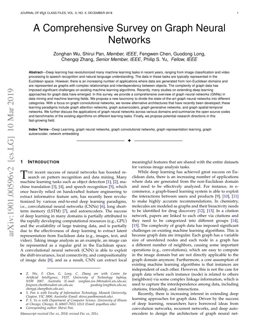The deep learning approaches for network embedding at the same time belong to graph neural networks, which include graph autoencoder-based algorithms (e.g., DNGR [42] and SDNE [43]) and graph convolution neural networks with unsuper- vised training(e.g., GraphSage [25]). Figure 2 describes the differences between network embedding and graph neural

JOURNAL OF LATEX CLASS FILES, VOL. X, NO. X, DECEMBER 2018 3 TABLE 1: Commonly used notations. Descriptions The length of a set Element-wise product. Transpose of vector/matrix A. Concatenation of A and B. A graph The set of nodes in a graph A node vi ∈ V The neighbors of node v The set of edges in a graph An edge eij ∈ E Notations | · | AT [A, B] G V vi N (v) E eij X ∈ RN×D The feature matrix of a graph. x ∈ RN Xi ∈ RD N M D T The feature vector of a graph in the case of D = 1. The feature vector of the node vi. The number of nodes, N = |V|. The number of edges, M = |E|. The dimension of a node vector. The total number of time steps in time series. Fig. 2: Network Embedding v.s. Graph Neural Networks. networks in this paper. Our Contributions Our paper makes notable contribu- tions summarized as follows: • New taxonomy In light of the increasing number of studies on deep learning for graph data, we propose a new taxonomy of graph neural networks (GNNs). 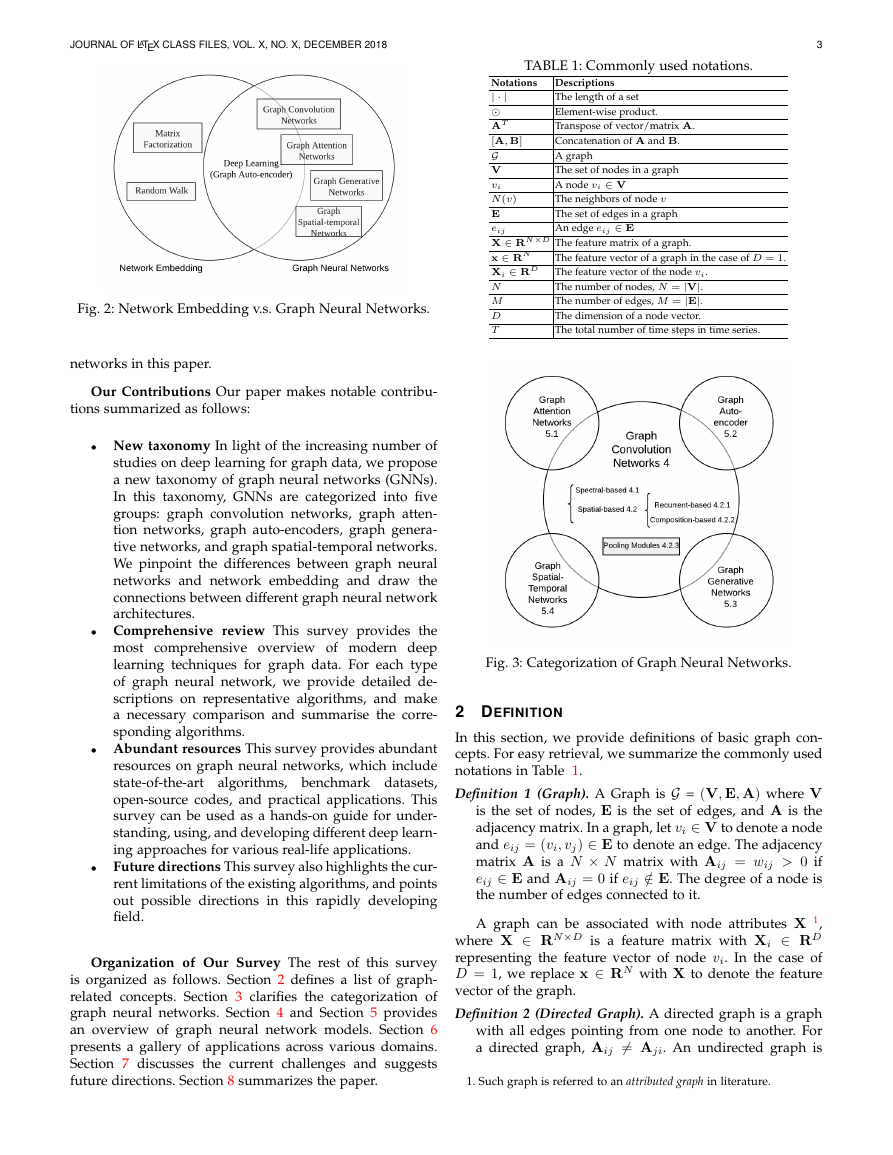In this taxonomy, GNNs are categorized into ﬁve groups: graph convolution networks, graph atten- tion networks, graph auto-encoders, graph genera- tive networks, and graph spatial-temporal networks. We pinpoint the differences between graph neural networks and network embedding and draw the connections between different graph neural network architectures. • Comprehensive review This survey provides the most comprehensive overview of modern deep learning techniques for graph data. For each type of graph neural network, we provide detailed de- scriptions on representative algorithms, and make a necessary comparison and summarise the corre- sponding algorithms. • Abundant resources This survey provides abundant resources on graph neural networks, which include state-of-the-art algorithms, benchmark datasets, open-source codes, and practical applications. This survey can be used as a hands-on guide for under- standing, using, and developing different deep learn- ing approaches for various real-life applications. Future directions This survey also highlights the cur- rent limitations of the existing algorithms, and points out possible directions in this rapidly developing ﬁeld. • Organization of Our Survey The rest of this survey is organized as follows. Section 2 deﬁnes a list of graph- related concepts. Section 3 clariﬁes the categorization of graph neural networks. Section 4 and Section 5 provides an overview of graph neural network models. Section 6 presents a gallery of applications across various domains. Section 7 discusses the current challenges and suggests future directions. Section 8 summarizes the paper. Fig. 3: Categorization of Graph Neural Networks. 2 DEFINITION In this section, we provide deﬁnitions of basic graph con- cepts. For easy retrieval, we summarize the commonly used notations in Table 1. Deﬁnition 1 (Graph). A Graph is G = (V, E, A) where V is the set of nodes, E is the set of edges, and A is the adjacency matrix. In a graph, let vi ∈ V to denote a node and eij = (vi, vj) ∈ E to denote an edge. The adjacency matrix A is a N × N matrix with Aij = wij > 0 if eij ∈ E and Aij = 0 if eij /∈ E. The degree of a node is the number of edges connected to it. A graph can be associated with node attributes X 1, where X ∈ RN×D is a feature matrix with Xi ∈ RD representing the feature vector of node vi. In the case of D = 1, we replace x ∈ RN with X to denote the feature vector of the graph. Deﬁnition 2 (Directed Graph). A directed graph is a graph with all edges pointing from one node to another. For a directed graph, Aij = Aji. An undirected graph is 1. Such graph is referred to an attributed graph in literature.

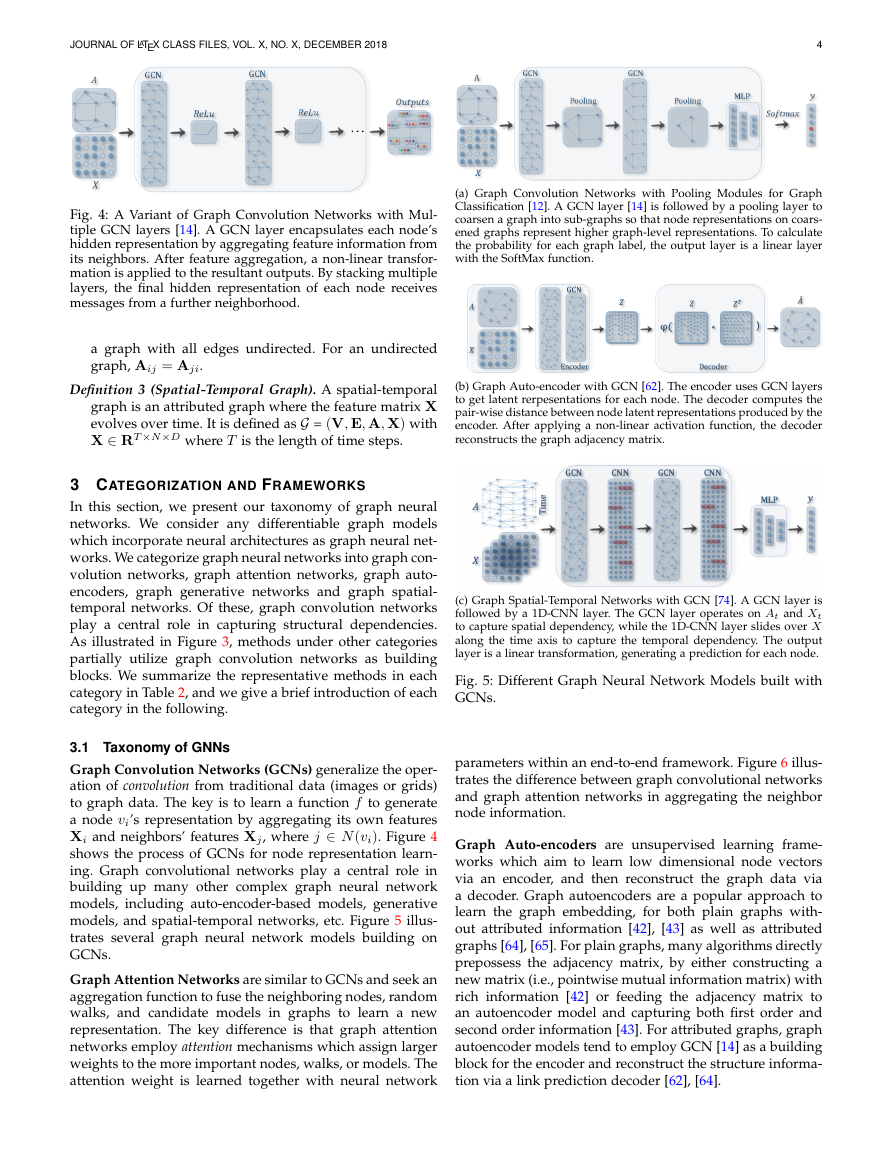
JOURNAL OF LATEX CLASS FILES, VOL. X, NO. X, DECEMBER 2018 4 (a) Graph Convolution Networks with Pooling Modules for Graph Classiﬁcation [12]. A GCN layer [14] is followed by a pooling layer to coarsen a graph into sub-graphs so that node representations on coars- ened graphs represent higher graph-level representations. To calculate the probability for each graph label, the output layer is a linear layer with the SoftMax function. Fig. 4: A Variant of Graph Convolution Networks with Mul- tiple GCN layers [14]. A GCN layer encapsulates each node’s hidden representation by aggregating feature information from its neighbors. After feature aggregation, a non-linear transfor- mation is applied to the resultant outputs. By stacking multiple layers, the ﬁnal hidden representation of each node receives messages from a further neighborhood. a graph with all edges undirected. For an undirected graph, Aij = Aji. Deﬁnition 3 (Spatial-Temporal Graph). A spatial-temporal graph is an attributed graph where the feature matrix X evolves over time. It is deﬁned as G = (V, E, A, X) with X ∈ RT×N×D where T is the length of time steps. (b) Graph Auto-encoder with GCN [62]. The encoder uses GCN layers to get latent rerpesentations for each node. The decoder computes the pair-wise distance between node latent representations produced by the encoder. After applying a non-linear activation function, the decoder reconstructs the graph adjacency matrix. 3 CATEGORIZATION AND FRAMEWORKS In this section, we present our taxonomy of graph neural networks. We consider any differentiable graph models which incorporate neural architectures as graph neural net- works. We categorize graph neural networks into graph con- volution networks, graph attention networks, graph auto- encoders, graph generative networks and graph spatial- temporal networks. Of these, graph convolution networks play a central role in capturing structural dependencies. As illustrated in Figure 3, methods under other categories partially utilize graph convolution networks as building blocks. We summarize the representative methods in each category in Table 2, and we give a brief introduction of each category in the following. 3.1 Taxonomy of GNNs Graph Convolution Networks (GCNs) generalize the oper- ation of convolution from traditional data (images or grids) to graph data. The key is to learn a function f to generate a node vi’s representation by aggregating its own features Xi and neighbors’ features Xj, where j ∈ N (vi). Figure 4 shows the process of GCNs for node representation learn- ing. Graph convolutional networks play a central role in building up many other complex graph neural network models, including auto-encoder-based models, generative models, and spatial-temporal networks, etc. Figure 5 illus- trates several graph neural network models building on GCNs. Graph Attention Networks are similar to GCNs and seek an aggregation function to fuse the neighboring nodes, random walks, and candidate models in graphs to learn a new representation. The key difference is that graph attention networks employ attention mechanisms which assign larger weights to the more important nodes, walks, or models. The attention weight is learned together with neural network (c) Graph Spatial-Temporal Networks with GCN [74]. A GCN layer is followed by a 1D-CNN layer. The GCN layer operates on At and Xt to capture spatial dependency, while the 1D-CNN layer slides over X along the time axis to capture the temporal dependency. The output layer is a linear transformation, generating a prediction for each node. Fig. 5: Different Graph Neural Network Models built with GCNs. 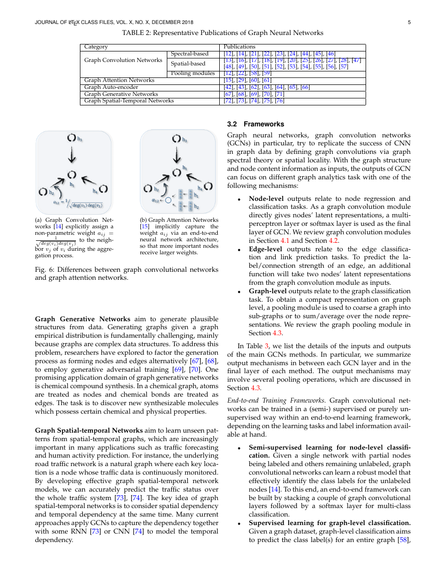parameters within an end-to-end framework. Figure 6 illus- trates the difference between graph convolutional networks and graph attention networks in aggregating the neighbor node information. Graph Auto-encoders are unsupervised learning frame- works which aim to learn low dimensional node vectors via an encoder, and then reconstruct the graph data via a decoder. Graph autoencoders are a popular approach to learn the graph embedding, for both plain graphs with- out attributed information [42], [43] as well as attributed graphs [64], [65]. For plain graphs, many algorithms directly prepossess the adjacency matrix, by either constructing a new matrix (i.e., pointwise mutual information matrix) with rich information [42] or feeding the adjacency matrix to an autoencoder model and capturing both ﬁrst order and second order information [43]. For attributed graphs, graph autoencoder models tend to employ GCN [14] as a building block for the encoder and reconstruct the structure informa- tion via a link prediction decoder [62], [64].

JOURNAL OF LATEX CLASS FILES, VOL. X, NO. X, DECEMBER 2018 5 TABLE 2: Representative Publications of Graph Neural Networks Category Graph Convolution Networks Graph Attention Networks Graph Auto-encoder Graph Generative Networks Graph Spatial-Temporal Networks Spectral-based Spatial-based Pooling modules (a) Graph Convolution Net- works [14] explicitly assign a non-parametric weight aij = √ to the neigh- bor vj of vi during the aggre- gation process. deg(vi)deg(vj ) 1 (b) Graph Attention Networks [15] implicitly capture the weight aij via an end-to-end neural network architecture, so that more important nodes receive larger weights. Fig. 6: Differences between graph convolutional networks and graph attention networks. Graph Generative Networks aim to generate plausible structures from data. Generating graphs given a graph empirical distribution is fundamentally challenging, mainly because graphs are complex data structures. To address this problem, researchers have explored to factor the generation process as forming nodes and edges alternatively [67], [68], to employ generative adversarial training [69], [70]. One promising application domain of graph generative networks is chemical compound synthesis. In a chemical graph, atoms are treated as nodes and chemical bonds are treated as edges. The task is to discover new synthesizable molecules which possess certain chemical and physical properties. Graph Spatial-temporal Networks aim to learn unseen pat- terns from spatial-temporal graphs, which are increasingly important in many applications such as trafﬁc forecasting and human activity prediction. For instance, the underlying road trafﬁc network is a natural graph where each key loca- tion is a node whose trafﬁc data is continuously monitored. By developing effective graph spatial-temporal network models, we can accurately predict the trafﬁc status over the whole trafﬁc system [73], [74]. The key idea of graph spatial-temporal networks is to consider spatial dependency and temporal dependency at the same time. Many current approaches apply GCNs to capture the dependency together with some RNN [73] or CNN [74] to model the temporal dependency. Publications [12], [14], [21], [22], [23], [24], [44], [45], [46] [13], [16], [17], [18], [19], [20], [25], [26], [27], [28], [47] [48], [49], [50], [51], [52], [53], [54], [55], [56], [57] [12], [22], [58], [59] [15], [29], [60], [61] [42], [43], [62], [63], [64], [65], [66] [67], [68], [69], [70], [71] [72], [73], [74], [75], [76] 3.2 Frameworks Graph neural networks, graph convolution networks (GCNs) in particular, try to replicate the success of CNN in graph data by deﬁning graph convolutions via graph spectral theory or spatial locality. With the graph structure and node content information as inputs, the outputs of GCN can focus on different graph analytics task with one of the following mechanisms: • Node-level outputs relate to node regression and classiﬁcation tasks. As a graph convolution module directly gives nodes’ latent representations, a multi- perceptron layer or softmax layer is used as the ﬁnal layer of GCN. We review graph convolution modules in Section 4.1 and Section 4.2. • Edge-level outputs relate to the edge classiﬁca- tion and link prediction tasks. To predict the la- bel/connection strength of an edge, an additional function will take two nodes’ latent representations from the graph convolution module as inputs. • Graph-level outputs relate to the graph classiﬁcation task. To obtain a compact representation on graph level, a pooling module is used to coarse a graph into sub-graphs or to sum/average over the node repre- sentations. We review the graph pooling module in Section 4.3. 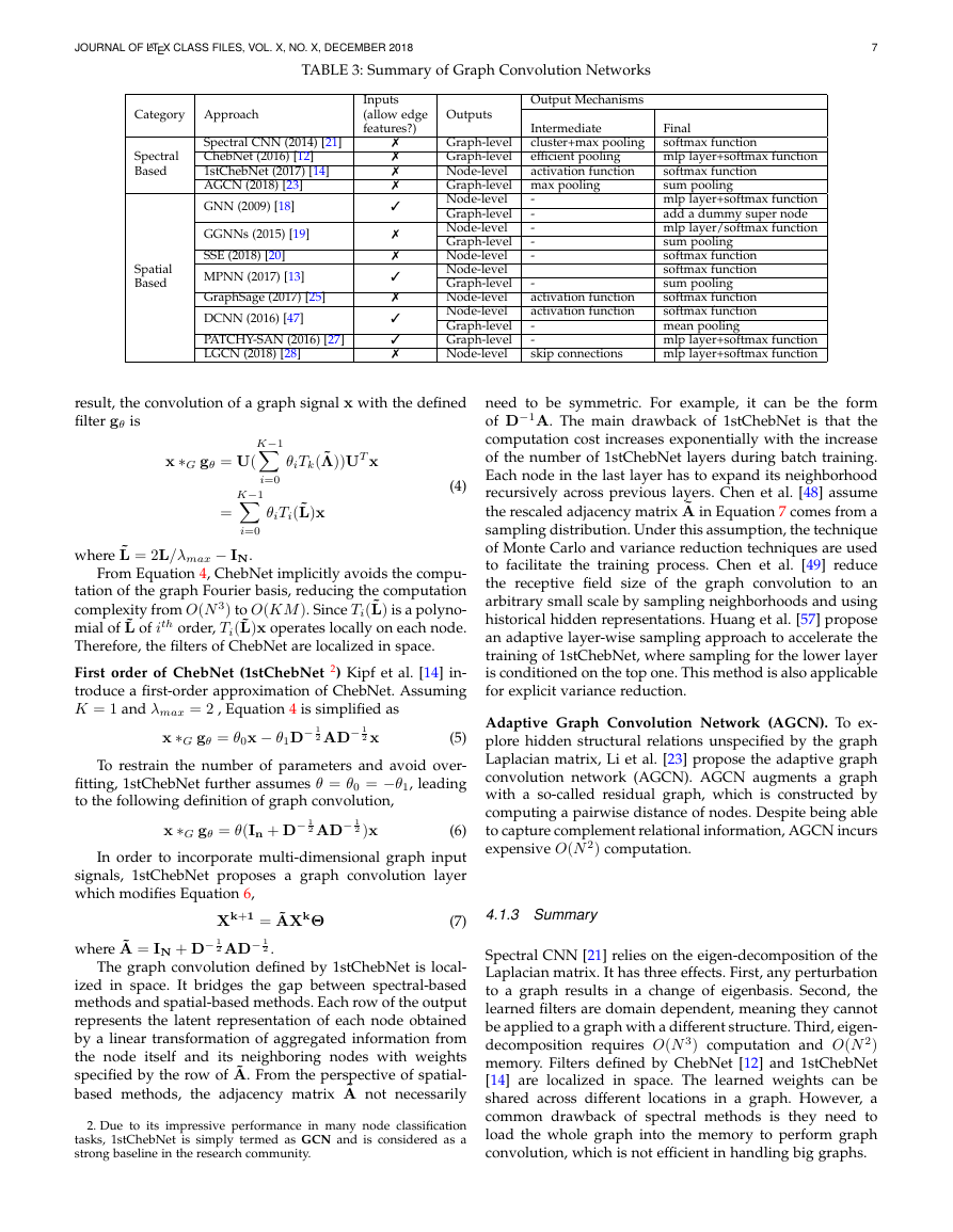In Table 3, we list the details of the inputs and outputs of the main GCNs methods. In particular, we summarize output mechanisms in between each GCN layer and in the ﬁnal layer of each method. The output mechanisms may involve several pooling operations, which are discussed in Section 4.3. End-to-end Training Frameworks. Graph convolutional net- works can be trained in a (semi-) supervised or purely un- supervised way within an end-to-end learning framework, depending on the learning tasks and label information avail- able at hand. • Semi-supervised learning for node-level classiﬁ- cation. Given a single network with partial nodes being labeled and others remaining unlabeled, graph convolutional networks can learn a robust model that effectively identify the class labels for the unlabeled nodes [14]. To this end, an end-to-end framework can be built by stacking a couple of graph convolutional layers followed by a softmax layer for multi-class classiﬁcation. • Supervised learning for graph-level classiﬁcation. Given a graph dataset, graph-level classiﬁcation aims to predict the class label(s) for an entire graph [58],

JOURNAL OF LATEX CLASS FILES, VOL. X, NO. X, DECEMBER 2018 [59], [77], [78]. The end-to-end learning for this task can be done with a framework which combines both graph convolutional layers and the pooling procedure [58], [59]. Speciﬁcally, by applying graph convolutional layers, we obtain representation with a ﬁxed number of dimensions for each node in every single graph. Then, we can get the representation of an entire graph through pooling which summarizes the representation vectors of all nodes in a graph. Finally, by applying linear layers and a softmax layer, we can build an end-to-end framework for graph classiﬁcation. An example is given in Fig 5a. • Unsupervised learning for graph embedding. When no class labels are available in graphs, we can learn the graph embedding in a purely unsupervised way in an end-to-end framework. These algorithms ex- ploit edge-level information in two ways. One simple way is to adopt an autoencoder framework where the encoder employs graph convolutional layers to embed the graph into the latent representation upon which a decoder is used to reconstruct the graph structure [62], [64]. Another way is to utilize the neg- ative sampling approach which samples a portion of node pairs as negative pairs while existing node pairs with links in the graphs being positive pairs. Then a logistic regression layer is applied after the convolutional layers for end-to-end learning [25]. 4 GRAPH CONVOLUTION NETWORKS In this section, we review graph convolution networks (GCNs), the fundamental of many complex graph neural network models. GCNs approaches fall into two categories, spectral-based and spatial-based. Spectral-based approaches deﬁne graph convolutions by introducing ﬁlters from the perspective of graph signal processing [79] where the graph convolution operation is interpreted as removing noise from graph signals. Spatial-based approaches formulate graph convolutions as aggregating feature information from neighbors. While GCNs operate on the node level, graph pooling modules can be interleaved with the GCN layer, to coarsen graphs into high-level sub-structures. As shown in Fig 5a, such an architecture design can be used to extract graph-level representations and to perform graph classiﬁ- cation tasks. In the following, we introduce spectral-based GCNs, spatial-based GCNs, and graph pooling modules separately. 4.1 Spectral-based Graph Convolutional Networks Spectral-based methods have a solid foundation in graph signal processing [79]. We ﬁrst give some basic knowledge background of graph signal processing, after which we review the representative research on the spectral-based GCNs. 4.1.1 Backgrounds In spectral-based models, graphs are assumed to be undi- rected. A robust mathematical representation of an undi- rected graph is the normalized graph Laplacian matrix, 6 2 AD− 1 deﬁned as L = In − D− 1 matrix of node degrees, Dii = 2 , where D is a diagonal j(Ai,j). The normalized graph Laplacian matrix possesses the property of being real symmetric positive semideﬁnite. With this property, the nor- malized Laplacian matrix can be factored as L = UΛUT , where U = [u0, u1,··· , un−1] ∈ RN×N is the matrix of eigenvectors ordered by eigenvalues and Λ is the diagonal matrix of eigenvalues, Λii = λi. The eigenvectors of the normalized Laplacian matrix form an orthonormal space, in mathematical words, UT U = I. In graph signal processing, a graph signal x ∈ RN is a feature vector of the nodes of a graph where xi is the value of the ith node. The graph Fourier transform to a signal x is deﬁned as F (x) = UT x and the in- verse graph Fourier transform is deﬁned as F −1(ˆx) = Uˆx, where ˆx represents the resulting signal from graph Fourier transform. To understand graph Fourier transform, from its deﬁnition we see that it indeed projects the input graph signal to the orthonormal space where the basis is formed by eigenvectors of the normalized graph Laplacian. Elements of the transformed signal ˆx are the coordinates of the graph signal in the new space so that the input signal can be i ˆxiui, which is exactly the inverse graph Fourier transform. Now the graph convolution of the input signal x with a ﬁlter g ∈ RN is deﬁned as represented as x = x ∗G g = F −1(F (x) F (g)) = U(UT x UT g) (1) where denotes the Hadamard product. If we denote a ﬁlter as gθ = diag(UT g), then the graph convolution is simpliﬁed as x ∗G gθ = UgθUT x (2) Spectral-based graph convolution networks all follow this deﬁnition. The key difference lies in the choice of the ﬁlter gθ. 4.1.2 Methods of Spectral-based GCNs fk−1 Spectral CNN. Bruna et al. [21] propose the ﬁrst spectral convolution neural network (Spectral CNN). Assuming the ﬁlter gθ = Θk i,j is a set of learnable parameters and consid- ering graph signals of multi-dimension, they deﬁne a graph convolution layer as Xk+1 :,j = σ( UΘk i,jUT Xk :,i) (j = 1, 2,··· , fk) (3) i=1 where Xk ∈ RN×fk−1 is the input graph signal, N is the number of nodes, fk−1 is the number of input channels and fk is the number of output channels, Θk i,j is a diagonal matrix ﬁlled with learnable parameters, and σ is a non- linear transformation. gθ = K−1 Chebyshev Spectral CNN (ChebNet). Defferrard et al. [12] propose ChebNet which deﬁnes a ﬁlter as Chebyshev polynomials of the diagonal matrix of eigenvalues, i.e, i=0 θiTk( ˜Λ), where ˜Λ = 2Λ/λmax − IN. The Chebyshev polynomials are deﬁned recursively by Tk(x) = 2xTk−1(x) − Tk−2(x) with T0(x) = 1 and T1(x) = x. As a

JOURNAL OF LATEX CLASS FILES, VOL. X, NO. X, DECEMBER 2018 7 TABLE 3: Summary of Graph Convolution Networks Category Approach Spectral Based Spatial Based Spectral CNN (2014) [21] ChebNet (2016) [12] 1stChebNet (2017) [14] AGCN (2018) [23] GNN (2009) [18] GGNNs (2015) [19] SSE (2018) [20] MPNN (2017) [13] GraphSage (2017) [25] DCNN (2016) [47] PATCHY-SAN (2016) [27] LGCN (2018) [28] Inputs (allow edge features?) Output Mechanisms Outputs Intermediate cluster+max pooling efﬁcient pooling activation function Graph-level Graph-level Node-level Graph-level max pooling Node-level Graph-level Node-level Graph-level Node-level Node-level Graph-level Node-level Node-level Graph-level Graph-level Node-level - activation function activation function - - skip connections - - - - - Final softmax function mlp layer+softmax function softmax function sum pooling mlp layer+softmax function add a dummy super node mlp layer/softmax function sum pooling softmax function softmax function sum pooling softmax function softmax function mean pooling mlp layer+softmax function mlp layer+softmax function result, the convolution of a graph signal x with the deﬁned ﬁlter gθ is K−1 x ∗G gθ = U( K−1 where ˜L = 2L/λmax − IN. i=0 i=0 = θiTk( ˜Λ))UT x (4) θiTi(˜L)x need to be symmetric. For example, it can be the form of D−1A. The main drawback of 1stChebNet is that the computation cost increases exponentially with the increase of the number of 1stChebNet layers during batch training. Each node in the last layer has to expand its neighborhood recursively across previous layers. Chen et al. [48] assume the rescaled adjacency matrix ˜A in Equation 7 comes from a sampling distribution. Under this assumption, the technique of Monte Carlo and variance reduction techniques are used to facilitate the training process. Chen et al. [49] reduce the receptive ﬁeld size of the graph convolution to an arbitrary small scale by sampling neighborhoods and using historical hidden representations. Huang et al. [57] propose an adaptive layer-wise sampling approach to accelerate the training of 1stChebNet, where sampling for the lower layer is conditioned on the top one. This method is also applicable for explicit variance reduction. Adaptive Graph Convolution Network (AGCN). To ex- plore hidden structural relations unspeciﬁed by the graph Laplacian matrix, Li et al. [23] propose the adaptive graph convolution network (AGCN). AGCN augments a graph with a so-called residual graph, which is constructed by computing a pairwise distance of nodes. Despite being able to capture complement relational information, AGCN incurs expensive O(N 2) computation. From Equation 4, ChebNet implicitly avoids the compu- tation of the graph Fourier basis, reducing the computation complexity from O(N 3) to O(KM ). Since Ti(˜L) is a polyno- mial of ˜L of ith order, Ti(˜L)x operates locally on each node. Therefore, the ﬁlters of ChebNet are localized in space. First order of ChebNet (1stChebNet 2) Kipf et al. [14] in- troduce a ﬁrst-order approximation of ChebNet. Assuming K = 1 and λmax = 2 , Equation 4 is simpliﬁed as x ∗G gθ = θ0x − θ1D− 1 2 AD− 1 2 x (5) To restrain the number of parameters and avoid over- ﬁtting, 1stChebNet further assumes θ = θ0 = −θ1, leading to the following deﬁnition of graph convolution, x ∗G gθ = θ(In + D− 1 2 AD− 1 2 )x (6) In order to incorporate multi-dimensional graph input signals, 1stChebNet proposes a graph convolution layer which modiﬁes Equation 6, where ˜A = IN + D− 1 Xk+1 = ˜AXkΘ 2 AD− 1 2 . 4.1.3 Summary (7) The graph convolution deﬁned by 1stChebNet is local- ized in space. It bridges the gap between spectral-based methods and spatial-based methods. Each row of the output represents the latent representation of each node obtained by a linear transformation of aggregated information from the node itself and its neighboring nodes with weights speciﬁed by the row of ˜A. From the perspective of spatial- based methods, the adjacency matrix ˜A not necessarily 2. Due to its impressive performance in many node classiﬁcation tasks, 1stChebNet is simply termed as GCN and is considered as a strong baseline in the research community. Spectral CNN [21] relies on the eigen-decomposition of the Laplacian matrix. It has three effects. First, any perturbation to a graph results in a change of eigenbasis. Second, the learned ﬁlters are domain dependent, meaning they cannot be applied to a graph with a different structure. Third, eigen- decomposition requires O(N 3) computation and O(N 2) memory. Filters deﬁned by ChebNet [12] and 1stChebNet [14] are localized in space. The learned weights can be shared across different locations in a graph. However, a common drawback of spectral methods is they need to load the whole graph into the memory to perform graph convolution, which is not efﬁcient in handling big graphs.

JOURNAL OF LATEX CLASS FILES, VOL. X, NO. X, DECEMBER 2018 8 rium is reached. To handle heterogeneous graphs, the spatial graph convolution of GNNs is deﬁned as v = f (lv, lco[v], ht−1 ht ne [v], lne[v]) (8) where lv denotes the label attributes of node v, lco[v] denotes the label attributes of corresponding edges of node v, ht ne[v] denotes the hidden representations of node v’s neighbors at time step t, and lne[v] denotes the label attributes of node v’s neighbors. To ensure convergence, the recurrent function f (·) must be a contraction mapping, which shrinks the distance be- tween two points after mapping. In the case of f (·) is a neural network, a penalty term has to be imposed on the Jacobian matrix of parameters. GNNs uses the Almeida- Pineda algorithm [80], [81] to train its model. The core idea is to run the propagation process to reach ﬁxed points and then perform the backward procedure given the converged solution. Gated Graph Neural Networks (GGNNs) employs gated recurrent units(GRU) [82] as the recurrent function, reduc- ing the recurrence to a ﬁxed number of steps. The spatial graph convolution of GGNNs is deﬁned as v = GRU (ht−1 ht v , Wht u) (9) u∈N (v) Different from GNNs, GGNNs use back-propagation through time (BPTT) to learn the parameters. The advantage is that it no longer needs to constrain parameters to ensure convergence. However, the downside of training by BPTT is that it sacriﬁces efﬁciency both in time and memory. This is especially problematic for large graphs, as GGNNs need to run the recurrent function multiple times over all nodes, requiring intermediate states of all nodes to be stored in memory. Stochastic Steady-state Embedding (SSE). To improve the learning efﬁciency, the SSE algorithm [20] updates the node latent representations stochastically in an asynchronous fashion. As shown in Algorithm 1, SSE recursively estimates node latent representations and updates the parameters with sampled batch data. To ensure convergence to steady states, the recurrent function of SSE is deﬁned as a weighted average of the historical states and new states, t = (1 − α)hv t−1 + αW1σ(W2[xv, hv t−1, xu]]) [hu u∈N (v) (10) Though summing neighborhood information implicitly con- siders node degree, it remains questionable whether the scale of this summation affects the stability of this algorithm. 4.2.2 Composition Based Spatial GCNs Composition-based methods update the nodes’ representa- tions by stacking multiple graph convolution layers. Message Passing Neural Networks (MPNNs). Gilmer et al. [13] generalize several existing graph convolution networks including [12], [14], [19], [21], [56], [83], [84] into a uni- ﬁed framework named Message Passing Neural Networks (MPNNs). The MPNNs consists of two phases, the message passing phase and the readout phase. 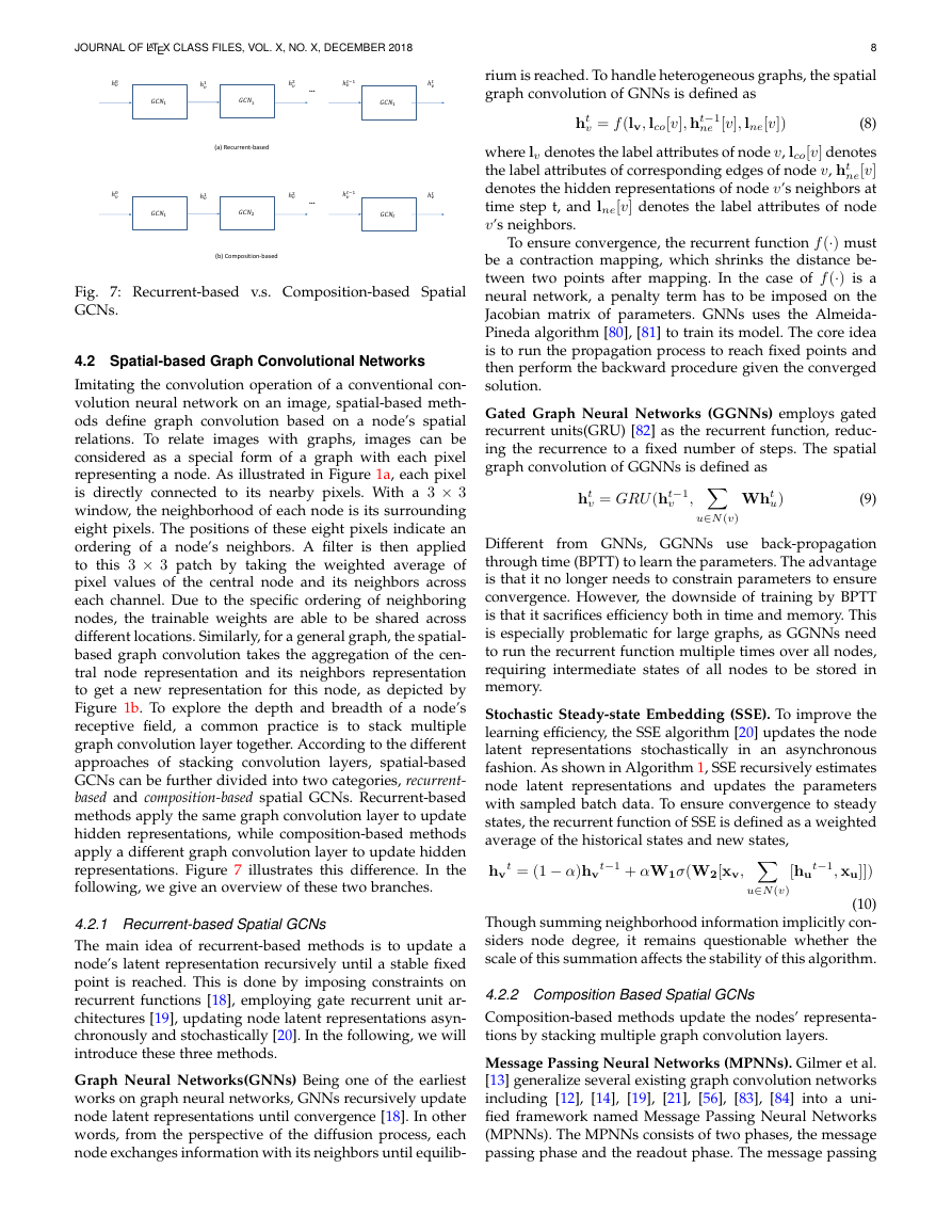The message passing Fig. 7: Recurrent-based v.s. Composition-based Spatial GCNs. 4.2 Spatial-based Graph Convolutional Networks Imitating the convolution operation of a conventional con- volution neural network on an image, spatial-based meth- ods deﬁne graph convolution based on a node’s spatial relations. To relate images with graphs, images can be considered as a special form of a graph with each pixel representing a node. As illustrated in Figure 1a, each pixel is directly connected to its nearby pixels. With a 3 × 3 window, the neighborhood of each node is its surrounding eight pixels. The positions of these eight pixels indicate an ordering of a node’s neighbors. A ﬁlter is then applied to this 3 × 3 patch by taking the weighted average of pixel values of the central node and its neighbors across each channel. Due to the speciﬁc ordering of neighboring nodes, the trainable weights are able to be shared across different locations. Similarly, for a general graph, the spatial- based graph convolution takes the aggregation of the cen- tral node representation and its neighbors representation to get a new representation for this node, as depicted by Figure 1b. To explore the depth and breadth of a node’s receptive ﬁeld, a common practice is to stack multiple graph convolution layer together. According to the different approaches of stacking convolution layers, spatial-based GCNs can be further divided into two categories, recurrent- based and composition-based spatial GCNs. Recurrent-based methods apply the same graph convolution layer to update hidden representations, while composition-based methods apply a different graph convolution layer to update hidden representations. Figure 7 illustrates this difference. In the following, we give an overview of these two branches. 4.2.1 Recurrent-based Spatial GCNs The main idea of recurrent-based methods is to update a node’s latent representation recursively until a stable ﬁxed point is reached. This is done by imposing constraints on recurrent functions [18], employing gate recurrent unit ar- chitectures [19], updating node latent representations asyn- chronously and stochastically [20]. In the following, we will introduce these three methods. Graph Neural Networks(GNNs) Being one of the earliest works on graph neural networks, GNNs recursively update node latent representations until convergence [18]. In other words, from the perspective of the diffusion process, each node exchanges information with its neighbors until equilib- !"#$!"#%!"#&…ℎ()ℎ($ℎ(%ℎ(&ℎ(&*$!"#$!"#$!"#$…ℎ()ℎ($ℎ(%ℎ(&ℎ(&*$(a) Recurrent-based(b) Composition-based

分享到：

赞收藏

资料库

A Comprehensive Survey on Graph Neural Network（2019）.pdf

相关推荐

人工智能

热门标签

最新资料