Theoretical Economics Letters, 2017, 7, 2213-2229
http://www.scirp.org/journal/tel
ISSN Online: 2162-2086
ISSN Print: 2162-2078
Risk Correlation Based on Time-Varying Copula
Function and Extreme Value Theory
Xinlong Ji1, Lu Zhou2,3*
1The School of Finance, Lanzhou University of Finance and Economics, Lanzhou, China
2Faculty of Business and Economics, Macquarie University, Sydney, Australia
3The School of Finance, Renmin University of China, Beijing, China
How to cite this paper: Ji, X.L. and Zhou, L.
(2017) Risk Correlation Based on Time-Varying
Copula Function and Extreme Value Theory.
Theoretical Economics Letters, 7, 2213-2229.
https://doi.org/10.4236/tel.2017.77151
Received: November 14, 2017
Accepted: December 15, 2017
Published: December 18, 2017
Copyright © 2017 by authors and
Scientific Research Publishing Inc.
This work is licensed under the Creative
Commons Attribution International
License (CC BY 4.0).
http://creativecommons.org/licenses/by/4.0/
Open Access
Abstract
The dependence structure of financial assets in financial risk measurement is
very important, the tail relations in particular. Authors of extant studies in
this field tended to focus on the linear analysis of the financial assets, rarely
considering nonlinear, asymmetric and thick-tail characteristics. Here, we ap-
ply the copulas connection function with time-varying factors to discuss the
risk dependency relationship between financial assets. Moreover, we develop
an SV-EVT model to fit variables’ marginal distribution combined with sto-
chastic volatility and extreme value theory. Finally, we present an empirical
comparative study of static and dynamic copula models applied to the sample
comprising of the Chinese mainland A-shares and Hong Kong stock market.
The results show that the CSJC copulas connection function describes the tail
features of stock index better than the normal copulas connection function.
Similarly, the time-varying model outperforms the static copulas model. Fur-
thermore, we observe an asymmetry dependence change rule between Chinese
mainland A-shares market and the Hong Kong stock market; the correlation
of lower tail is significantly higher than that of the upper tail, and the bear
market effect is remarkable. These findings indicate that time-varying Copu-
las-SV-EVT model can depict the correlation of financial asset tails exactly,
and can thus be used to control investment risk and forecast abnormal fluctu-
ations.
Keywords
Time-Varying Copula, SV-t-EVT Model, Risk, Correlation
1. Introduction
Owing to the rapid advances in the information technology, loose financial reg-
DOI: 10.4236/tel.2017.77151 Dec. 18, 2017
2213
Theoretical Economics Letters
�
X. L. Ji, L. Zhou
DOI: 10.4236/tel.2017.77151
ulation and capital operation innovation, the financial resource allocation and
capital flows have already surpassed the scope of national borders. Against the
background of financial globalization, the economic development of all countries
has become more closely interrelated, and fluctuated with each other in every
capital markets. As a result, the risk contagion of the financial markets has be-
come more serious, as is shown in a series of financial crises, starting with the
American subprime mortgage crisis, followed by the European sovereign debt
caused by the financial crisis in Greece, and culminating in the global dramatic
decrease in the price of gold caused by the rise in the USD exchange rate and the
alleviation of global inflation. In China’s stock market, since our financial indus-
try has started opening to the outside investors, the number and size of the QDII
and QFII funds has experienced rapid growth, albeit with the increasingly en-
hanced correlation with global stock market volatility. This not only undermines
the stability of the stock market itself, but also investor confidence. Risk diversi-
fication is the primary goal of diversified investment. However, achieving this
aim has become difficult due to the global financial crisis. The changes in the na-
ture of the stock market risk dependency have become a major concern for in-
vestors and regulators. Therefore, in this work, we examine risk contagion, fo-
cusing on the tail correlation. By measuring and comparing with the domestic capi-
tal market, we also provide some useful advice for financial regulators and all types
of investors.
In this research field, the widely used measures of contagious risks are corre-
lation coefficient method, the GARCH model, VAR co-integration as well as the
Granger Causality Test. However, these methods have some notable measure-
ment deficiencies [1] [2] [3], such as the insufficient depiction of non-linearity,
asymmetry as well as the related features of the tail of financial variations, or the
inadequate knowledge of the time-varying financial measurement. Copula, as a
connection function, can create a multivariate distribution with flexibility and
feasibility by connecting the marginal distribution of random variable and its
joint distribution. This, in turn, can show the non-linearity and dynamic features
better when analyzing the correlation between variables, thus effectively compen-
sating for the insufficiency associated with measuring traditional risk correlation.
Moreover, the copula function and its serial correlation indices can correctly and
easily present the tail correlation when analyzing samples of variables, which is an
obvious advantage relative to other widely used analytical computation methods.
This is particularly relevant when studying the financial market risk features, such
as the correlation among extreme risks and fluctuation overflow [4] [5]. Owing to
these advantageous characteristics, copula function is widely used in its many
forms, such as the Standard Copula, t-Copula, Gumbel Copula, Clayton Copula,
Frank Copula, etc. [6] [7]. However, copulas are primarily used in constant cor-
relation, while the correlation among financial variables is affected by market
fluctuations. Thus, using fixed correlation is incorrect in this context, especially
when the market is subject to some extreme events. The time-varying copula can
be used to describe the non-linear dependence of financial capital and that of the
2214
Theoretical Economics Letters
�
X. L. Ji, L. Zhou
tail and describe the dynamic structure of the financial capital better, due to its
consideration of the time-variation of parameters and their structures [8] [9]. Hence,
in this paper, we present a model of risk correlations based on the time-varying
copula.
The basic principle of copula is connecting the joint distribution function of
multiple random variables by the one-dimensional marginal distribution func-
tion. Given that the measure of an individual financial asset by the marginal dis-
tribution function itself shall influence the accuracy of the correlation of the final
variable, it is vital to obtain the marginal distribution function in order to cor-
rectly evaluate the risk of contagion. In practice, the patterning of capital fluctu-
ation is mainly performed via the GARCH model and random fluctuation in the
SV model. In particular, the former is easy to use and understand, and is thus
usually combined with copula theory when studying correlation of risks [10] [11]
[12]. However, the definite relationship between the financial capital profits and
fluctuation contained by the GARCH model cannot be proved theoretically [13].
In order to overcome this deficiency, some scholars combine the SV model with
copula theory when conducting analyses. In spite of the fact that Copula-SV is
seldom used in practical research, available evidence indicates that the SV model
is superior to GARCH in depicting financial data. Similarly, Copula-SV is pre-
ferable to Copula GARCH when the aim is to elucidate the risks pertaining to
joint investment [14]. Additionally, the SV model also has some deficiencies, such
as inability to identify extreme financial events, typically exhibited by the abnor-
mal data of the tail, despite its accuracy in depicting the fluctuation of financial
capital. Although the EVT can measure the risky losses in extremity for the tail
distribution of profits by GPD, it does not study the overall distribution of prof-
its. Moreover, in extreme conditions characterized by high risk, the empirical dis-
tribution by EVT is very close to reality, which is beyond the predictability of sam-
ples and can deal with the tail thick with effectiveness [15] [16] [17]. Given the
aforementioned facts, along with the abnormal distribution and tick tail of the
financial capital variables, in this study, we contribute to combine the SV and EVT
to depict and construct the joint distribution of samples in measuring the risks
of contagion of financial capital. Also, considering that Chinese market is one of
the biggest emerging markets which is different from developed market, this study
thus contributes to employ the data from both Chinese A-share market and Hong
Kong stock market to examine the theory by empirical testing the performance
in the emerging market.
In sum, in order to construct a joint model capable of reflecting the actual
distribution of all the financial capital variables and their correlative fluctuation,
which is necessary for measuring the contagious risks of related financial capital
with accuracy, our aim is to elucidate the marginal distribution of capital varia-
ble fluctuations by combining SV and EVT. In addition, this paper constructs a
financial chronological correlation by combining time-varying copula theory in
order to develop a new model—a time-varying Copula-SV-EVT—for measuring
the correlation between risks pertaining to financial capital. The data utilized in
2215
Theoretical Economics Letters
DOI: 10.4236/tel.2017.77151
�
X. L. Ji, L. Zhou
model verification comprise of Hushen 300 Index and the Hang Seng Index of
Hong Kong. More specifically, after establishing the correlation of risks in the
two markets, suggestions for investment institutions are provided. The remainder
of this paper is organized as follows: In Section 2, we apply the acquisition of the
research samples to elaborate the time-varying copula theory and its marginal
distribution. Section 3 introduces the development of the time-varying Copu-
la-SV-EVT model and its parameter estimates. In Section 4, the analysis of the
data features is presented, along with the empirical test of the model. Section 5
concludes this paper.
2. Time-Varying Copula Theory
2.1. Basic Theory of Copula Function
The theoretical work on copulas dates back to Sklar’s research in 1959, who
holds that a joint distribution can be divided into K marginal distributions and a
copula function, which depicts the correlation among the variables. Copula function
]
0,1
can be considered a multi-dimensionally distributed function
,
F evenly allocated in the [0,1] range.
with its marginal distribution
More specifically, let A denote a joint distribution function in N dimensions,
(
(
F x F x
F x
,
. Then, there exists a copula function C in accordance
n
2
(
F x x
,
with the equation:
. In addition, if
1
2
(
(
F x F x
F x
,
are constantly distributed, the copula function is defi-
n
2
F is a
nite. Otherwise, if function C is n-dimensional copula, and 1
distributed function, function F is n-dimensional random variable joint distribu-
tion function.
(
(
C F x F x
2
[
]
: 0,1
(
F x
n
)
=
x
n
,
F F
1
2
,
F F
2
,
)
)
→
)
,
)
,
)
,
)
,
)
,
,
)
)
(
(
)
,
1
n
(
,
n
,
,
,
C
n
[
1
1
,
Furthermore, the Copula theory provides a simple method for constructing a
model of complex and multiple variables and is conducive to the analysis and
understanding of many financial problems. There are three main applications of
Copula in Finance: the multi-derivative asset pricing, financial risk management
and credit risk management. Cherubini, Luciano and Vecchiato have extended
the application of Copulas to all fields of finance [18]. In their study, they em-
phatically researched the frontier issues about the market synergies, credit deriv-
atives pricing, hedging and risk management. From the perspective of probabil-
ity, they applied the Copula function into these areas and discussed the applica-
tions in the fields of the credit derivative assets (credit-default swaps, CDOs) and
multi-asset options pricing (binary digital option, rainbow option, fragile and
barrier options) in detail. In addition, Bouyé et al. and Durrleman et al. also
made great contributions in introducing the Copulas into the finance area [19]
[20].
2.2. Time-Varying Copula Function
The traditional correlation index of multi-dimensional variables is often de-
picted by liner correlation. However, this correlation obviously has some limita-
tions [21], because fluctuations vary according to conditions, whereby the corre-
2216
Theoretical Economics Letters
DOI: 10.4236/tel.2017.77151
�
X. L. Ji, L. Zhou
lation between variables inevitably changes. This is particularly the case for fi-
nancial markets subject to sudden and extensive changes. Such abnormal fluctu-
ations in the market cannot be described via liner correlation. Consequently, the
time-varying correlation model should be employed when describing the tail.
The tail correlation description allows establishing whether another significant
market fluctuation shall be evoked by an earlier occurrence of a similar fluctua-
tion. Copula function is particularly appropriate for establishing the correlation
),C u v does exist, the lower tail correlation and the upper
of the tail. If copula
tail correlation of the financial capital variables can be expressed as follows:
(
L
τ
=
lim
u
0
→
C u u
,
(
)
u
,
U
τ
=
lim
u
1
→
1 2
−
(
u C u u
,
+
1
−
u
)
(1)
However, there are many copulas, each with distinct characteristics. For exam-
ple, the Standard Copula and the t-Copula cannot depict the asymmetry of the
financial capital; Gumbel Copula fails to grasp the lower tail correlation; Clayton
Copula fails to grasp the upper tail correlation; Frank Copula cannot establish
both the upper and the lower tail correlation; while compared with the common
Copula, the JC Copula is superior in describing both the upper and the lower tail
correlation. Nevertheless, it is affected by the asymmetry in describing the joint
distribution of the same correlation in both the upper and the lower tail. To over-
come this deficiency, Patton [8] proposed SJC Copula. This function has been
widely used in the correlation calculations pertaining to the financial market and
financial capital. In this work, we also adopt the time-varying SJC-Copula as the
connecting function, described as follows:
C
+
1
(2)
In practice, when studying the tail correlation of the financial chronological
Uτ and
sequences by using copula function, the relevant parameters of the tail
Lτ are assumed to be constant for simplicity. However, assuming that fluctua-
tions in the financial market are constant, the correlation of the sequences in
fluctuation is obtained in relation to time. In order to highlight the feature of con-
stant variation, a process similar to ARMA can be used to describe the correla-
tion of the upper and the lower tail of SJC-Copula [22]. The function equation is
given below:
C u v
,
JC
+ + −
L
τ τ
L
τ τ
L
τ τ
u v
C
SJC
u v
,
0.5
(
1
,1
=
−
−
u
(
)
(
)
)
v
JC
U
U
U
,
,
,
j
j
j
−
j
L
U
1
=
10
10
+
+
+
+
u
t
= ∧
= ∧
∑
L
L t
1
−
ν
−
t
−
U
U t
1
−
1
10
1
10
ω βτ α
L
ω βτ α
U
(3)
L
τ
t
U
τ
t
(
( )
Lτ remain in the [−1,1]
x∧
1 e
= −
where
Lτ are the two parameters measuring the dynamic structure of
Uτ and
range,
the tail, and thus characterize the time-variation function. These parameters and the
tail correlation parameters of the time-varying function SJC-Copula have one-to-one
correspondence, thus allowing the asymmetry, the tail feature as well as the cor-
guarantees that Uτ and
) (
ν
−
t
−
1 e
+
∑
u
t
)
1
=
−
x
j
j
x
DOI: 10.4236/tel.2017.77151
2217
Theoretical Economics Letters
�
X. L. Ji, L. Zhou
relation of the market subject to severe fluctuation to be described.
3. The Construction of the Marginal Distribution Model
The adoption of the marginal distribution is justified by the correlation of finan-
cial capital measured by the copula function and the features of the peak of the
thick tail and different variance. In this work, we develop the SV-t-EVT model,
which allows depicting the marginal distribution of profits of joint capital invest-
ments. This is achieved by depicting the fluctuation of profits of individual capi-
tal investments, followed by measuring the conditional variance to obtain the indi-
vidual random disturbance terms after filtration, and finally constructing the model
of the upper and lower tail of the random disturbance terms based on the POT
pattern of the extreme value theory.
3.1. SV-t Model and Its Filtration of Random Disturbance Terms
SV-t model is an expansion of the basic SV model. It represents the thick tail of
the capital profits more realistically and has a greater ability to discern the fluc-
tuation in these profits. Consequently [11], in this work, we adopt SV-t model to
depict the fluctuation of profits of individual capital investments, described by
the following equation:
(
θ ε ε
t
(
)
y
i i d t
=
~ . .
t
,
θ µ φθ µ η η
+
t
(
)
0,1,
υ
i i d N
~ . .
(4)
exp
= +
)2
τ
)
−
0,
=
1,2,
,
n
,
t
(
2
t
,
t
t
t
1
−
t
tε and
where residual term
tη are independent; φ is a constant parameter,
embodying the impact of the current fluctuation on that in the future; when
1φ < , the covariance is stable. Compared with the basic SV model, in the SV-t
model,
tε is subjected to the distribution of t with a υ degrees of freedom.
This is preferred to standard normal distribution, which reflects the features of
financial capital variables—insubordination to the standard distribution of the
time series. In order to acquire the samples of a series of random disturbance terms,
it is necessary to evaluate the SV-t model parameters. The commonly used me-
thods for evaluating parameters are QML (pseudo maximum likelihood method)
and GMM (generalized method of moments), resulting in a greater error in the
parameter evaluation for their limits on the condition of the samples. Although
the method based on MCMC (Markov Chain Monte Carlo) is highly complex, the
parameter estimation is quite accurate [23]. MCMC does not require the analyt-
ical expression of posterior density, but provides a method to sample the para-
meter vector from the posterior distribution. This method sets a Markov Chain,
equating its stationary distribution to the posterior density. When the Markov
Chain is self-restrained, the value of simulation is supposed to be samples taken
from posterior distribution. Therefore, in this work, we apply the MCMC of the
Gibbs samples to evaluate parameters by using the SV-t model via the BUGS soft-
ware.
2218
Theoretical Economics Letters
DOI: 10.4236/tel.2017.77151
�
X. L. Ji, L. Zhou
3.2. Extreme Value Theory and SV-t Marginal Distribution Model
The fluctuation of capital profits is depicted by applying the SV-t model, thereby
ˆtµ and
obtaining a series of random disturbance terms
ˆtσ denote the conditional average value and conditional variance of capital profits
series, respectively:
tZ after filtration. Let
(
Z
,
,
Z
t
)
t n
1
− +
X
=
−
ˆ
µ
t n
1
− +
t n
1
− +
ˆ
σ
t n
1
− +
,
,
ˆ
µ
t
X
−
t
ˆ
σ
t
(5)
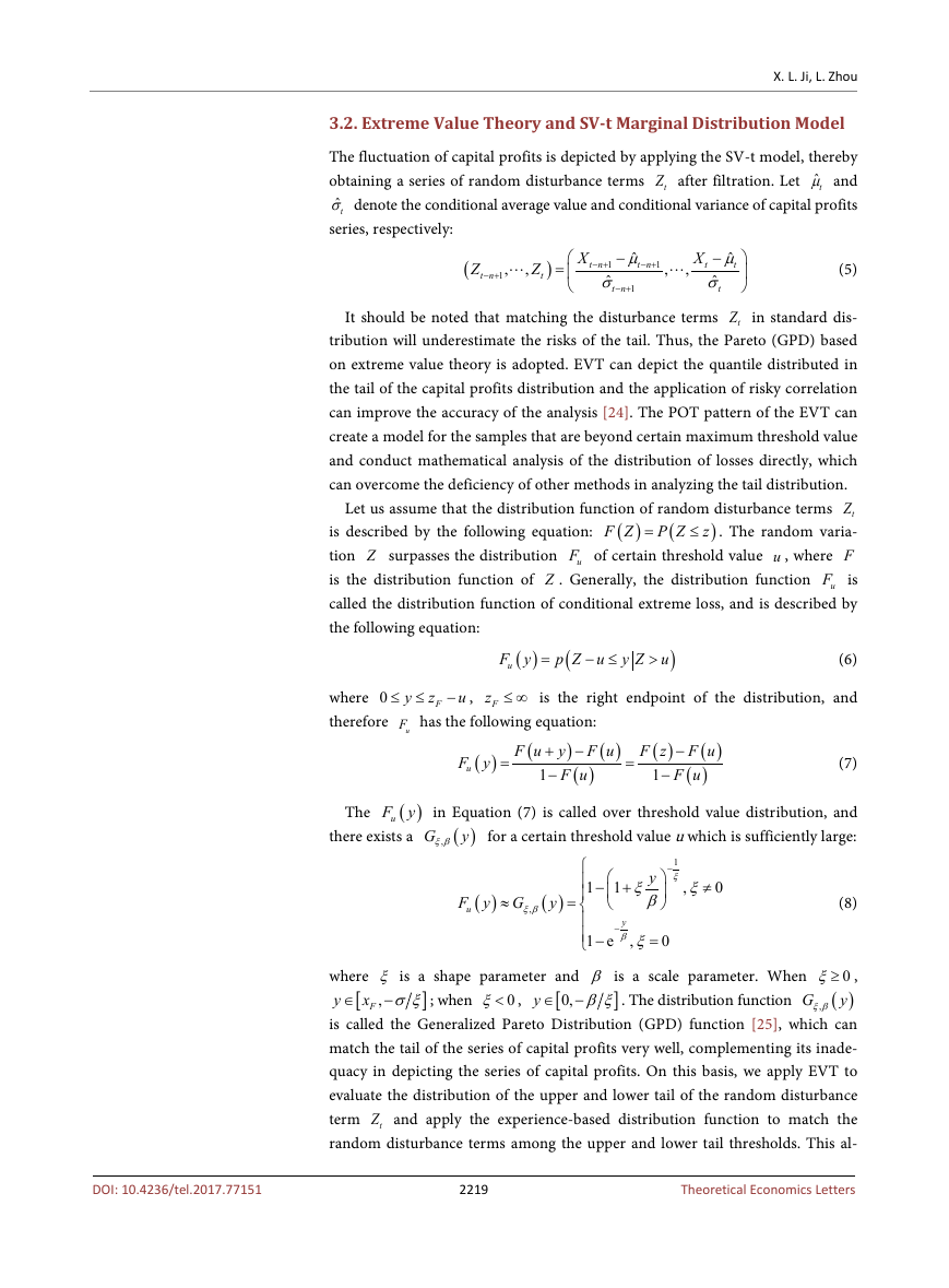
It should be noted that matching the disturbance terms
tZ in standard dis-
tribution will underestimate the risks of the tail. Thus, the Pareto (GPD) based
on extreme value theory is adopted. EVT can depict the quantile distributed in
the tail of the capital profits distribution and the application of risky correlation
can improve the accuracy of the analysis [24]. The POT pattern of the EVT can
create a model for the samples that are beyond certain maximum threshold value
and conduct mathematical analysis of the distribution of losses directly, which
can overcome the deficiency of other methods in analyzing the tail distribution.
tZ
is described by the following equation:
. The random varia-
uF of certain threshold value u , where F
tion Z surpasses the distribution
uF is
is the distribution function of Z . Generally, the distribution function
called the distribution function of conditional extreme loss, and is described by
the following equation:
Let us assume that the distribution function of random disturbance terms
(
F Z
(
P Z
=
≤
)
)
z
(
uF y
)
=
(
p Z u
− ≤
y Z u
>
)
(6)
where 0
therefore
F
z
u
− ,
y
≤ ≤
uF has the following equation:
( )
F u
Fz ≤ ∞ is the right endpoint of the distribution, and
(
F y
u
)
=
(
F u
+
1
−
)
y
−
( )
F u
=
( )
F z
1
−
( )
F u
−
( )
F u
(7)
The
)
(
there exists a
uF y in Equation (7) is called over threshold value distribution, and
for a certain threshold value u which is sufficiently large:
y
(
)
,G
ξβ
F y G
u
≈
(
)
ξβ
,
(
y
)
=
1
−
ξ
+
ξ
y
β
,
ξ
≠
0
(8)
1
−
1
−
1 e
−
y
β
,
ξ
=
0
[
y
−
∈
0,
]
βξ
0ξ< ,
; when
[
∈ −
]
x σξ
,F
. The distribution function
where ξ is a shape parameter and β is a scale parameter. When
0ξ≥ ,
)
y
,G
ξβ
is called the Generalized Pareto Distribution (GPD) function [25], which can
match the tail of the series of capital profits very well, complementing its inade-
quacy in depicting the series of capital profits. On this basis, we apply EVT to
evaluate the distribution of the upper and lower tail of the random disturbance
tZ and apply the experience-based distribution function to match the
term
random disturbance terms among the upper and lower tail thresholds. This al-
y
(
DOI: 10.4236/tel.2017.77151
2219
Theoretical Economics Letters
�
X. L. Ji, L. Zhou
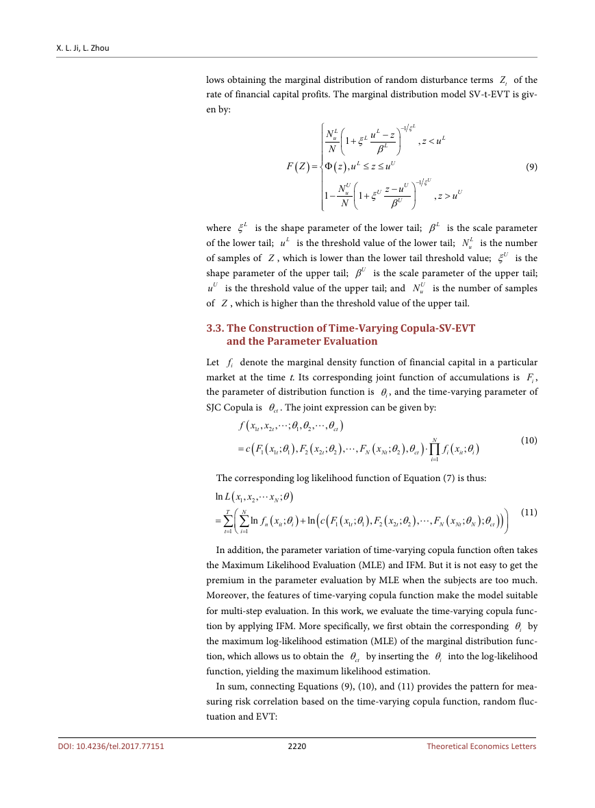
tZ of the
lows obtaining the marginal distribution of random disturbance terms
rate of financial capital profits. The marginal distribution model SV-t-EVT is giv-
en by:
(
F Z
)
+
1
L
N
u
N
= Φ
( )
z u
,
1
U
N
u
N
−
L
ξ
L
u
−
z
L
β
z u
≤ ≤
U
L
1
−
L
ξ
,
z u
<
L
(9)
1
+
U
ξ
U
z u
−
U
β
1
−
U
ξ
,
z
>
U
u
Lu is the threshold value of the lower tail;
Lξ is the shape parameter of the lower tail;
where
of the lower tail;
of samples of Z , which is lower than the lower tail threshold value;
shape parameter of the upper tail;
Uu is the threshold value of the upper tail; and
of Z , which is higher than the threshold value of the upper tail.
Lβ is the scale parameter
uN is the number
Uξ is the
Uβ is the scale parameter of the upper tail;
uN is the number of samples
U
L
3.3. The Construction of Time-Varying Copula-SV-EVT
and the Parameter Evaluation
if denote the marginal density function of financial capital in a particular
iF ,
iθ, and the time-varying parameter of
Let
market at the time t. Its corresponding joint function of accumulations is
the parameter of distribution function is
SJC Copula is
,
ctθ . The joint expression can be given by:
(
f x
x
t
1
2
(
(
c F x
t
1
(10)
;
θ
i
)
,
(
F x
2
2
;
θ θ θ
ct
1
;
θ θ
ct
(
F x
N
(
f x
i
it
)
)
;
θ
2
;
θ
1
=
)
)
)
Nt
,
,
,
,
,
,
,
2
1
2
t
t
N
⋅∏
i
1
=
The corresponding log likelihood function of Equation (7) is thus:
ln
)
;
θ
x
,
N
(
f
n
x
it
;
θ
i
)
+
ln
(
(
(
c F x
t
1
1
;
θ
1
)
,
(
F x
2
2
t
;
θ
2
)
,
,
(
F x
N
Nt
;
θ θ
ct
;
N
)
(11)
)
)
(
L x x
,
1
2
T
N
∑ ∑
1
=
1
=
t
i
ln
=
In addition, the parameter variation of time-varying copula function often takes
the Maximum Likelihood Evaluation (MLE) and IFM. But it is not easy to get the
premium in the parameter evaluation by MLE when the subjects are too much.
Moreover, the features of time-varying copula function make the model suitable
for multi-step evaluation. In this work, we evaluate the time-varying copula func-
tion by applying IFM. More specifically, we first obtain the corresponding
iθ by
the maximum log-likelihood estimation (MLE) of the marginal distribution func-
tion, which allows us to obtain the
iθ into the log-likelihood
ctθ by inserting the
function, yielding the maximum likelihood estimation.
In sum, connecting Equations (9), (10), and (11) provides the pattern for mea-
suring risk correlation based on the time-varying copula function, random fluc-
tuation and EVT:
2220
Theoretical Economics Letters
DOI: 10.4236/tel.2017.77151
�




 2023年江西萍乡中考道德与法治真题及答案.doc
 2012年重庆南川中考生物真题及答案.doc
 2013年江西师范大学地理学综合及文艺理论基础考研真题.doc
 2020年四川甘孜小升初语文真题及答案I卷.doc
 2020年注册岩土工程师专业基础考试真题及答案.doc
 2023-2024学年福建省厦门市九年级上学期数学月考试题及答案.doc
 2021-2022学年辽宁省沈阳市大东区九年级上学期语文期末试题及答案.doc
 2022-2023学年北京东城区初三第一学期物理期末试卷及答案.doc
 2018上半年江西教师资格初中地理学科知识与教学能力真题及答案.doc
 2012年河北国家公务员申论考试真题及答案-省级.doc
 2020-2021学年江苏省扬州市江都区邵樊片九年级上学期数学第一次质量检测试题及答案.doc
 2022下半年黑龙江教师资格证中学综合素质真题及答案.doc