Open economies review 12: 265–280, 2001
c 2001 Kluwer Academic Publishers. Printed in The Netherlands.
Trade Flows and Spatial Effects:
The Gravity Model Revisited
A. POROJAN
A.Porojan@Bradford.ac.uk; anca@porojan.freeserve.co.uk
University of Bradford, Development and Project Planning Centre, Pemberton Building, Bradford,
BD7 1DP, UK
Key words: spatial econometrics, trade forecasting, gravity model
JEL Classification Numbers: F17, R15
Abstract
This article revisits the popular gravity model of trade in light of the increasingly acknowledged
findings of spatial econometrics and interprets the results in view of some recent theoretical devel-
opments from the economic literature that contribute to its foundation. When the inherent spatial
effects are explicitly taken into account, the magnitude of the estimated parameters changes con-
siderably and, with it, the measures on the predicted trade flows. This result is illustrated for the
case of predicted trade flows between the European Union and some of its potential members.
Introduction
Given its parsimony and often acclaimed empirical robustness, the gravity
model of trade has never lost its appeal over the nearly four decades since
it was introduced by Tinbergen (1962) and Linnemann (1966).
Indeed, the late 1990s witnessed a revival in its application, with numerous
authors employing it to assess the potential for trade between the European
Union (EU) and the transforming economies of Central and Eastern Europe.
Since Krugman (1991), the fact that geography matters where trade is con-
cerned is no longer news. However, the empirical work on the gravity model
of trade does not, to date, explicitly account for the role of location, and nei-
ther does it take seriously Anselin and Griffith’s (1988) exposition on ways in
which standard econometric techniques fail to remain applicable in the spatial
context.
This article explores the empirical performance of the gravity model when
the inherent spatial effects are explicitly accounted for within the framework
of spatial econometrics. The emphasis is on the size and significance of the
estimated parameters,1 given the practical relevance of the calculated poten-
tial trade flows they generate. We find that, when the inherent spatial effects
are explicitly taken into account, the magnitude of the estimated parameters
�
266
POROJAN
changes considerably and, with it, the measures on the predicted trade flows.
More specifically, the traditional formulation seriously overestimates the size
of the trade flows to and from “island” countries, while underestimating it for
countries that have trading neighbors. Moreover, the large explanatory power
of regional trading bloc membership dummy variables vanishes when spatial
effects are included in the model specification. The overall performance of the
alternative specification proposed is superior to the one of the currently pre-
vailing formulation.
The article is structured in three sections. The first section presents the tra-
ditional gravity model and the reasons to revisit it, and is followed by details of
the proposed specification and the corresponding empirical results (Section 2).
Section 3 concludes.
1. The prevailing specification
1.1. Formulation
The gravity model belongs to the class of empirical models concerned with the
determinants of interaction. In its most general formulation, it explains a flow Fi j
(of goods, people etc.) from an area i to an area j as a function of characteristics
of the origin .Oi /, characteristics of the destination .D j / and some separation
measurement .Si j /:
Fi j D Oi D j Si j ;
i D 1; : : : ; II j D 1; : : : ; J:
(1)
Customarily, the model is estimated in log-linear form.
The inspiration for the formulation comes from Newtonian physics (Zhang and
Kristensen, 1995, p. 308) and more specifically from the law of universal gravity,
according to which attraction is larger between larger and more closely posi-
tioned bodies. When applied to flows of goods between countries, by analogy,
the model stresses that trade increases with size and proximity of the trading
partners.
Rewriting (1) in log form, a vector of bilateral trade flows (exports, imports,
total trade) Fi j is modeled as
Fi j D Xfl C ";
" » N .0; 2/;
(2)
where X is a vector of (logs of) explanatory variables, and " is a white-noise
error term.
In the simplest specification, X contains proxies for the size of the two
economies (GDP, population and/or GDP per capita) and the distance between
them (as proxy for transportation costs and other obstacles to trade). Some
models include, alongwith distance, the areas of the trading partners (proxy
for transport cost within the country), tariff and price variables, and a variety
�
TRADE FLOWS AND SPATIAL EFFECTS
267
of proxies for “closeness” between the trading partners: contiguity, common
language dummy (cultural affinity), trading bloc membership dummy, etc. (see
Zhang and Kristensen, 1995, for an overview), and even FDI as a comple-
ment/substitute to/for trade (Fontagn ´e, Freudenberg and Pajot, 1999).
Most familiar uses of the model relate to the examination of bilateral trade
patterns in search of evidence on “natural” (noninstitutional) regional trading
blocs (Frankel, Stein, and Wei, 1995; Frankel, 1998); the estimation of trade
creation and trade diversion effects from regional integration (e.g., Brada and
M ´endez, 1985; Frankel, 1998; Endoh, 1999); the estimation of trade potential,
with application to trade between the European Union and its potential members
(e.g., Hamilton and Winters, 1992; Baldwin, 1994, and references therein; Gros
and Steinherr, 1995;2 Brulhart and Kelly, 1999).
1.2. Limitations
Despite its empirical success, the gravity model has not been free from criti-
cism. A frequent complaint relates to its lack of theoretical foundations (e.g.,
Leamer, 1994)—a view no longer prevalent, however (Baldwin, 1994), in light of
several recent developments. Evenett and Keller (1998) show that much of the
success of the gravity equation relies on theories of trade based on increasing
returns to scale. Evenett and Keller’s analysis is, however, focused on the pro-
portionality of the volume of trade to the trading countries’ incomes and not on
the relationship of volume of trade to trade resistance or on the role of the de-
mand side. Concentrating more on the role of distance, Asilis and Rivera-Batiz
(1994) develop a geographical theory of interregional trade in which space plays
a central role. As far as the role of demand is concerned, the predominant rele-
vant argument remains the Linder hypothesis, according to which differences in
taste deter trade due to the cost of tailoring a product to the local requirements;
this hypothesis is usually interpreted in the sense that the intensity of bilateral
trade decreases with differences in per capita income (Leamer, 1994).
While reviewing similar contributions (either largely empirical or more formal
ones, in the context of product differentiation and monopolistic competition),
Deardorff (1998) reconciles the gravity model with the classical theories of trade,
showing how the equation can be derived from a factor endowment model.
Most relevant to our line of argument—namely, that location matters—are
two particular developments: the papers of Asilis and Rivera-Batiz (1994) and
Bougheas, Demetriades and Morgenroth (1999). The first paper extends and
formalizes the basic elements of the gravity model, making location an en-
dogenous variable and examining how trade is brought about by the inter-
action between size, distance, and divergent regional productive structures
(p. 357). Essentially, in this model trade occurs as a result of the endogenous
geographical dispersion of factors of production and population (p. 372); in
other words, what makes regions different from each other is their location in
space. The second paper introduces infrastructure in the bilateral trade model
�
268
POROJAN
and shows that location and endowment (income) play a decisive role in de-
termining whether two partner countries will decide to enhance their trading
opportunities by developing (transport-cost reducing) infrastructure. The latter
has the features of an international public good, with spillovers from the country
investing in infrastructure and with multilateral benefits (i.e., a reduction in trans-
action costs with all trading partners for both the investing countries and their
neighbors).
Grossman (1998) brings together the old and new theories of trade with ref-
erence to the gravity equation. The explanatory power of the income variables
for the trading partner countries is, he argues, due to specialization, and “of
course some degree of specialization is at the heart of any model of trade”
(p. 29). In the presence of specialization, a larger income of the importing coun-
try corresponds to a larger ability to buy, while a larger output (income) of the
exporting country means a larger quantity available for consumers in the im-
porting country—irrespective of the supply-side considerations that gave rise
to the specialization (p. 30). The use of distance as a proxy for transport costs in
particular and transaction costs in general has both theoretical relevance and
empirical appeal. Grossman (1998) agrees with the anticipated and estimated
negative relationship between bilateral trade flows and distance but questions
the size of the estimated parameter (p. 30).
Also at the empirical level, Polak (1996) is concerned with the misspecifica-
tion and built-in bias (downward for “far-away countries” and upward for “close-
by countries,” p. 538). He is joined by one of the discussants of Hamilton and
Winters (1992) in calling for “a more differentiated measure of distance” (p. 109).
This point is taken up by Frankel and Wei (1998) and Brulhart and Kelly (1999),
who include in their ordinary least squares (OLS) estimation a remoteness indi-
cator (calculated as the average of a country’s distances to its trading partners,
weighted by the partners’ income).
Fik and Mulligan (1998) question the appropriateness of the widely used
“highly restrictive log-linear specifications” of gravity-type models and sug-
gest the use of Box–Cox transformations. Their results indicate that parameter
estimation bias comes from both inappropriate choice of explanatory variables
and functional misspecification.
Nevertheless, most authors continue to estimate and report OLS estimates
for a model of the type described in (2) above, ignoring the misspecification
caused by the nature of measurement problems associated with data collected
for aggregate spatial units and by the implications of violated standard assump-
tions that underlie their regression analysis.
A prominent example is Frankel (1998)—a valuable collection of both the-
oretical and empirical papers on the regionalization of the world economy. Its
opening chapter stresses that “many of the most interesting aspects of regional
trading arrangements require the introduction of a geographical dimension”
(p. 1), largely ignored in most of the past international trade research. However,
none of the empirical papers that follow the introduction accounts explicitly for
�
TRADE FLOWS AND SPATIAL EFFECTS
269
this dimension, thus continuing the tradition of reporting results obtained using
standard regression analysis applied to spatial data.
Anselin (1998) clarifies that such data are characterized by the presence of
spatial effects, namely, spatial dependence (caused by various degrees of spa-
tial aggregation, spatial externalities, and spillover effects) and spatial structure
or heteroskedasticity (resulting from “heterogeneity inherent in the delineation
of spatial units and from contextual variation over space,” p. 1). When such
effects are present, traditional econometric techniques are no longer applica-
ble, since spatial effects do, separately or in combination, impact upon the
properties of the traditional estimators and statistical tests.
In the presence of spatial effects, the appropriate technique is that of spatial
econometrics, which enables testing for multiple sources of misspecification in
spatial models and for spatial dependence when other forms of misspecification
are present (Anselin, 1998, p. 2), and which can deal with the multidirectional
nature of spatial dependence that often precludes the use of OLS.
2. Proposed specification
The application of standard econometrics techniques in the presence of spa-
tially correlated error terms results in misleading significance tests and mea-
sures of fit, due to biased estimation of error variance, t-test significance, and
R2. Ignoring spatial heterogeneity (structural instability and heteroskedasticity)
leads to biased parameter estimates and misleading significance levels (Anselin
and Griffith, 1988, pp. 16–17).
The two problems have not been totally ignored in the literature, but nei-
ther have they received full attention. While Baldwin (1994) overviews a set
of generic issues of empirical implementation of the OLS estimation, with no
mention of spatial effects, Bougheas, Demetriades, and Morgenroth (1999) ac-
knowledge the possibility of spatially autocorrelated error terms and use the
methodology of (instrumental variables) seemingly unrelated regression. How-
ever, for identical explanatory variables, OLS and generalized least squares
(GLS) are identical, and no gain in efficiency is obtained from the GLS estimation
(Greene, 2000, pp. 614–616). The problem of heteroskedasticity is addressed by
Flowerdew (1982), who suggests an iterative weighting method, and is acknowl-
edged by McCallum (1995), who opts for a weighted OLS regression. Zhang and
Kristensen (1995) and Poon (1995) also address the issue of heterogeneity and
propose a model with variable coefficients obtained by applying Casetti’s ex-
pansion method to a gravity-based trade model.3
2.1. Formulation
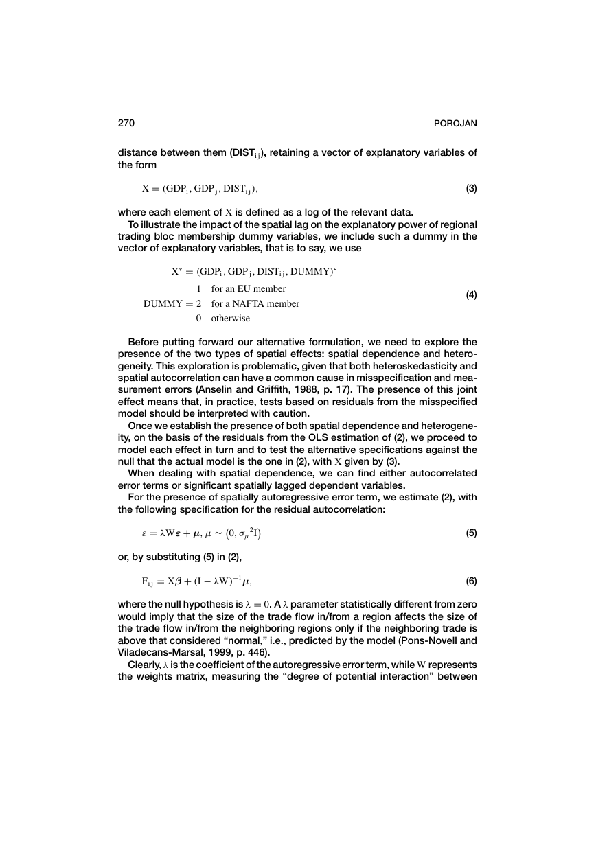
For the purpose of our comparative analysis, we model trade flows as a function
of income per capita (GDPi , GDP j ) in the trading partner countries and the
�
270
POROJAN
distance between them (DISTi j ), retaining a vector of explanatory variables of
the form
X D .GDPi ; GDP j ; DISTi j /;
(3)
where each element of X is defined as a log of the relevant data.
To illustrate the impact of the spatial lag on the explanatory power of regional
trading bloc membership dummy variables, we include such a dummy in the
vector of explanatory variables, that is to say, we use
⁄ D .GDPi ; GDP j ; DISTi j ; DUMMY/‘
X
1 for an EU member
DUMMY D 2 for a NAFTA member
0 otherwise
(4)
Before putting forward our alternative formulation, we need to explore the
presence of the two types of spatial effects: spatial dependence and hetero-
geneity. This exploration is problematic, given that both heteroskedasticity and
spatial autocorrelation can have a common cause in misspecification and mea-
surement errors (Anselin and Griffith, 1988, p. 17). The presence of this joint
effect means that, in practice, tests based on residuals from the misspecified
model should be interpreted with caution.
Once we establish the presence of both spatial dependence and heterogene-
ity, on the basis of the residuals from the OLS estimation of (2), we proceed to
model each effect in turn and to test the alternative specifications against the
null that the actual model is the one in (2), with X given by (3).
When dealing with spatial dependence, we can find either autocorrelated
error terms or significant spatially lagged dependent variables.
For the presence of spatially autoregressive error term, we estimate (2), with
the following specification for the residual autocorrelation:
" D ‚W" C „; „ »¡
0; „
2I
¢
(5)
or, by substituting (5) in (2),
Fi j D Xfl C .I ¡ ‚W/¡1„;
(6)
where the null hypothesis is ‚ D 0. A ‚ parameter statistically different from zero
would imply that the size of the trade flow in/from a region affects the size of
the trade flow in/from the neighboring regions only if the neighboring trade is
above that considered “normal,” i.e., predicted by the model (Pons-Novell and
Viladecans-Marsal, 1999, p. 446).
Clearly, ‚ is the coefficient of the autoregressive error term, while W represents
the weights matrix, measuring the “degree of potential interaction” between
�
TRADE FLOWS AND SPATIAL EFFECTS
271
neighboring locations (Anselin et al., 1996, p. 81). W can be specified in a variety
of ways (see, e.g., Bolduc, Laferri `ere, and Santarossa, 1992); here we use the
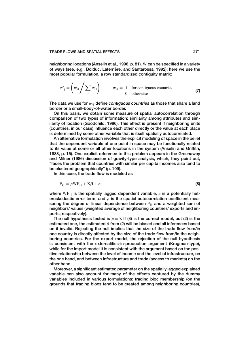
most popular formulation, a row standardized contiguity matrix:
ˆ
,X
!
w⁄
i j
D
wi j
wi j
j
wi j D 1
0
for contiguous countries
otherwise
(7)
The data we use for wi j define contiguous countries as those that share a land
border or a small-body-of-water border.
On this basis, we obtain some measure of spatial autocorrelation through
comparison of two types of information: similarity among attributes and sim-
ilarity of location (Goodchild, 1986). This effect is present if neighboring units
(countries, in our case) influence each other directly or the value at each place
is determined by some other variable that is itself spatially autocorrelated.
An alternative formulation involves the explicit modeling of space in the belief
that the dependent variable at one point in space may be functionally related
to its value at some or all other locations in the system (Anselin and Griffith,
1988, p. 15). One explicit reference to this problem appears in the Greenaway
and Milner (1986) discussion of gravity-type analysis, which, they point out,
“faces the problem that countries with similar per capita incomes also tend to
be clustered geographically” (p. 109).
In this case, the trade flow is modeled as
Fi j D ‰WFi j C Xfl C ";
(8)
is the spatially lagged dependent variable, " is a potentially het-
where WFi j
eroskedastic error term, and ‰ is the spatial autocorrelation coefficient mea-
suring the degree of linear dependence between Fi j and a weighted sum of
neighbors’ values (weighted average of neighboring countries’ exports and im-
ports, respectively).
The null hypothesis tested is ‰ D 0. If (8) is the correct model, but (2) is the
estimated one, the estimated fl from (2) will be biased and all inferences based
on it invalid. Rejecting the null implies that the size of the trade flow from/in
one country is directly affected by the size of the trade flow from/in the neigh-
boring countries. For the export model, the rejection of the null hypothesis
is consistent with the externalities-in-production argument (Krugman-type),
while for the import model it is consistent with the argument based on the pos-
itive relationship between the level of income and the level of infrastructure, on
the one hand, and between infrastructure and trade (access to markets) on the
other hand.
Moreover, a significant estimated parameter on the spatially lagged explained
variable can also account for many of the effects captured by the dummy
variables included in various formulations: trading bloc membership (on the
grounds that trading blocs tend to be created among neighboring countries),
�
272
POROJAN
linguistic (admittedly, not for the Commonwealth), and cultural affinities (again,
among neighbors), etc.
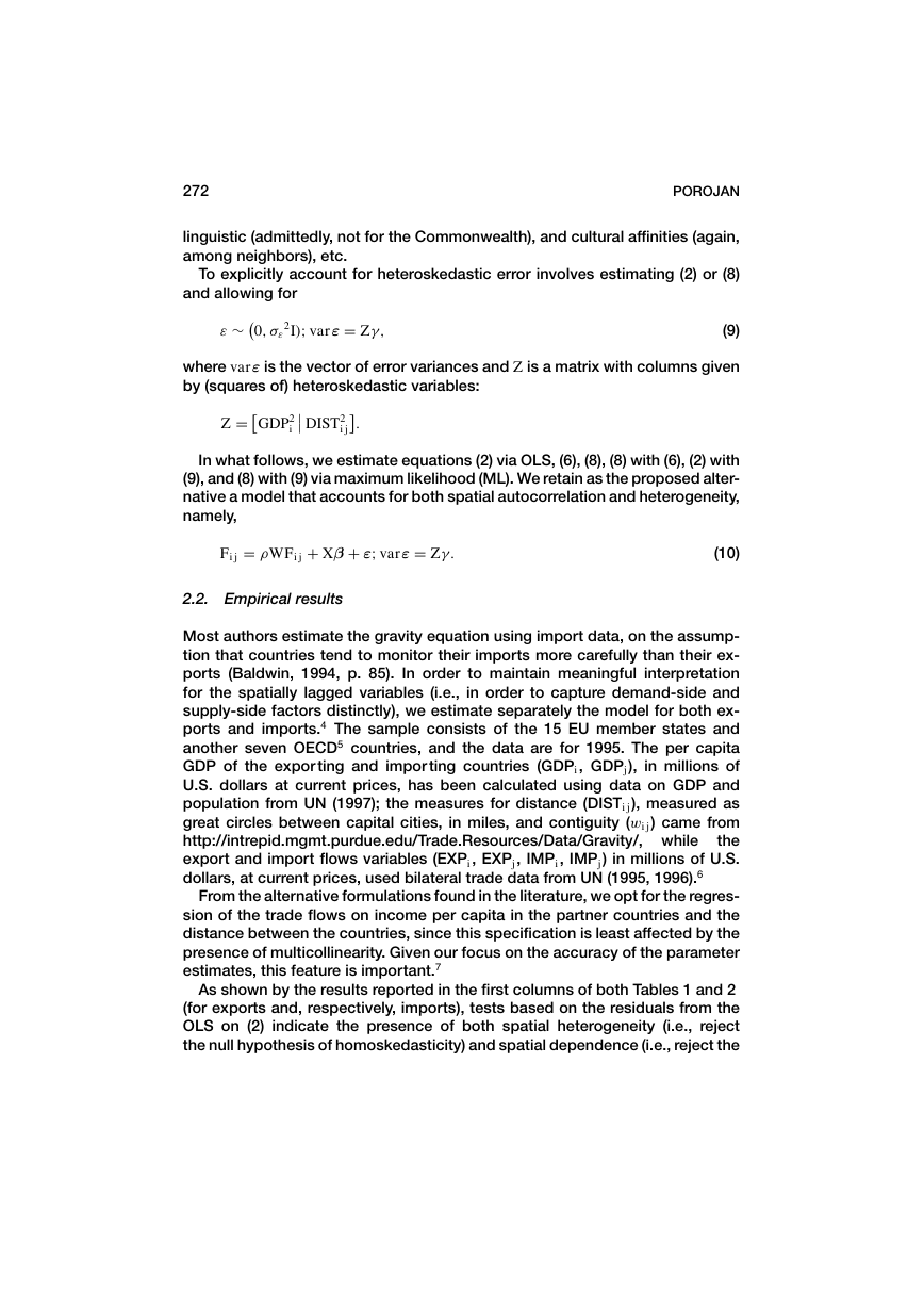
To explicitly account for heteroskedastic error involves estimating (2) or (8)
and allowing for
2I/I var" D Z ;
(9)
0; "
" »¡
Z D£
flfl DIST2
i j
⁄
:
GDP2
i
where var" is the vector of error variances and Z is a matrix with columns given
by (squares of) heteroskedastic variables:
In what follows, we estimate equations (2) via OLS, (6), (8), (8) with (6), (2) with
(9), and (8) with (9) via maximum likelihood (ML). We retain as the proposed alter-
native a model that accounts for both spatial autocorrelation and heterogeneity,
namely,
Fi j D ‰WFi j C Xfl C "I var" D Z :
(10)
2.2. Empirical results
Most authors estimate the gravity equation using import data, on the assump-
tion that countries tend to monitor their imports more carefully than their ex-
ports (Baldwin, 1994, p. 85). In order to maintain meaningful interpretation
for the spatially lagged variables (i.e., in order to capture demand-side and
supply-side factors distinctly), we estimate separately the model for both ex-
ports and imports.4 The sample consists of the 15 EU member states and
another seven OECD5 countries, and the data are for 1995. The per capita
GDP of the expor ting and impor ting countries (GDPi , GDPj ), in millions of
U.S. dollars at current prices, has been calculated using data on GDP and
population from UN (1997); the measures for distance (DISTi j ), measured as
great circles between capital cities, in miles, and contiguity (wi j ) came from
http://intrepid.mgmt.purdue.edu/Trade.Resources/Data/Gravity/, while
the
export and import flows variables (EXPi , EXPj , IMPi , IMPj ) in millions of U.S.
dollars, at current prices, used bilateral trade data from UN (1995, 1996).6
From the alternative formulations found in the literature, we opt for the regres-
sion of the trade flows on income per capita in the partner countries and the
distance between the countries, since this specification is least affected by the
presence of multicollinearity. Given our focus on the accuracy of the parameter
estimates, this feature is important.7
As shown by the results reported in the first columns of both Tables 1 and 2
(for exports and, respectively, imports), tests based on the residuals from the
OLS on (2) indicate the presence of both spatial heterogeneity (i.e., reject
the null hypothesis of homoskedasticity) and spatial dependence (i.e., reject the
�



 2023年江西萍乡中考道德与法治真题及答案.doc
 2012年重庆南川中考生物真题及答案.doc
 2013年江西师范大学地理学综合及文艺理论基础考研真题.doc
 2020年四川甘孜小升初语文真题及答案I卷.doc
 2020年注册岩土工程师专业基础考试真题及答案.doc
 2023-2024学年福建省厦门市九年级上学期数学月考试题及答案.doc
 2021-2022学年辽宁省沈阳市大东区九年级上学期语文期末试题及答案.doc
 2022-2023学年北京东城区初三第一学期物理期末试卷及答案.doc
 2018上半年江西教师资格初中地理学科知识与教学能力真题及答案.doc
 2012年河北国家公务员申论考试真题及答案-省级.doc
 2020-2021学年江苏省扬州市江都区邵樊片九年级上学期数学第一次质量检测试题及答案.doc
 2022下半年黑龙江教师资格证中学综合素质真题及答案.doc