【5】Very deep convolutional networks for large-scale image recogn....pdf

发布时间：2022-05-31 发布人：admin 分类：说明书资料大小：0.18M 资料格式：pdf 举报版权申诉

xinghaoyan-11614168-4744300845399354612.pdf-第1页.png

第1页 / 共14页

xinghaoyan-11614168-4744300845399354612.pdf-第2页.png

第2页 / 共14页

xinghaoyan-11614168-4744300845399354612.pdf-第3页.png

第3页 / 共14页

xinghaoyan-11614168-4744300845399354612.pdf-第4页.png

第4页 / 共14页

xinghaoyan-11614168-4744300845399354612.pdf-第5页.png

第5页 / 共14页

xinghaoyan-11614168-4744300845399354612.pdf-第6页.png

第6页 / 共14页

xinghaoyan-11614168-4744300845399354612.pdf-第7页.png

第7页 / 共14页

xinghaoyan-11614168-4744300845399354612.pdf-第8页.png

第8页 / 共14页

文本预览

5 1 0 2 r p A 0 1 ] V C . s c [ 6 v 6 5 5 1 . 9 0 4 1 : v i X r a Published as a conference paper at ICLR 2015 VERY DEEP CONVOLUTIONAL NETWORKS FOR LARGE-SCALE IMAGE RECOGNITION Karen Simonyan∗ & Andrew Zisserman+ Visual Geometry Group, Department of Engineering Science, University of Oxford {karen,az}@robots.ox.ac.uk ABSTRACT In this work we investigate the effect of the convolutional network depth on its accuracy in the large-scale image recognition setting. Our main contribution is a thorough evaluation of networks of increasing depth using an architecture with very small (3 × 3) convolution ﬁlters, which shows that a signiﬁcant improvement on the prior-art conﬁgurations can be achieved by pushing the depth to 16–19 weight layers. These ﬁndings were the basis of our ImageNet Challenge 2014 submission, where our team secured the ﬁrst and the second places in the localisa- tion and classiﬁcation tracks respectively. We also show that our representations generalise well to other datasets, where they achieve state-of-the-art results. We have made our two best-performing ConvNet models publicly available to facili- tate further research on the use of deep visual representations in computer vision. 1 INTRODUCTION Convolutional networks (ConvNets) have recently enjoyed a great success in large-scale im- age and video recognition (Krizhevsky et al., 2012; Zeiler & Fergus, 2013; Sermanet et al., 2014; Simonyan & Zisserman, 2014) which has become possible due to the large public image reposito- ries, such as ImageNet (Deng et al., 2009), and high-performance computing systems, such as GPUs or large-scale distributed clusters (Dean et al., 2012). In particular, an important role in the advance of deep visual recognition architectures has been played by the ImageNet Large-Scale Visual Recog- nition Challenge (ILSVRC) (Russakovsky et al., 2014), which has served as a testbed for a few generations of large-scale image classiﬁcation systems, from high-dimensional shallow feature en- codings (Perronnin et al., 2010) (the winner of ILSVRC-2011) to deep ConvNets (Krizhevsky et al., 2012) (the winner of ILSVRC-2012). With ConvNets becoming more of a commodity in the computer vision ﬁeld, a number of at- tempts have been made to improve the original architecture of Krizhevsky et al. (2012) in a bid to achieve better accuracy. For instance, the best-performing submissions to the ILSVRC- 2013 (Zeiler & Fergus, 2013; Sermanet et al., 2014) utilised smaller receptive window size and smaller stride of the ﬁrst convolutional layer. Another line of improvements dealt with training and testing the networks densely over the whole image and over multiple scales (Sermanet et al., 2014; Howard, 2014). In this paper, we address another important aspect of ConvNet architecture design – its depth. To this end, we ﬁx other parameters of the architecture, and steadily increase the depth of the network by adding more convolutional layers, which is feasible due to the use of very small (3 × 3) convolution ﬁlters in all layers. As a result, we come up with signiﬁcantly more accurate ConvNet architectures, which not only achieve the state-of-the-art accuracy on ILSVRC classiﬁcation and localisation tasks, but are also applicable to other image recognition datasets, where they achieve excellent performance even when used as a part of a relatively simple pipelines (e.g. deep features classiﬁed by a linear SVM without ﬁne-tuning). We have released our two best-performing models1 to facilitate further research. The rest of the paper is organised as follows. In Sect. 2, we describe our ConvNet conﬁgurations. The details of the image classiﬁcation training and evaluation are then presented in Sect. 3, and the ∗current afﬁliation: Google DeepMind +current afﬁliation: University of Oxford and Google DeepMind 1http://www.robots.ox.ac.uk/˜vgg/research/very_deep/ 1

Published as a conference paper at ICLR 2015 conﬁgurations are compared on the ILSVRC classiﬁcation task in Sect. 4. Sect. 5 concludes the paper. For completeness, we also describe and assess our ILSVRC-2014 object localisation system in Appendix A, and discuss the generalisation of very deep features to other datasets in Appendix B. Finally, Appendix C contains the list of major paper revisions. 2 CONVNET CONFIGURATIONS To measure the improvement brought by the increased ConvNet depth in a fair setting, all our ConvNet layer conﬁgurations are designed using the same principles, inspired by Ciresan et al. (2011); Krizhevsky et al. (2012). In this section, we ﬁrst describe a generic layout of our ConvNet conﬁgurations (Sect. 2.1) and then detail the speciﬁc conﬁgurations used in the evaluation (Sect. 2.2). Our design choices are then discussed and compared to the prior art in Sect. 2.3. 2.1 ARCHITECTURE During training, the input to our ConvNets is a ﬁxed-size 224 × 224 RGB image. The only pre- processing we do is subtracting the mean RGB value, computed on the training set, from each pixel. The image is passed through a stack of convolutional (conv.) layers, where we use ﬁlters with a very small receptive ﬁeld: 3 × 3 (which is the smallest size to capture the notion of left/right, up/down, center). In one of the conﬁgurations we also utilise 1 × 1 convolution ﬁlters, which can be seen as a linear transformation of the input channels (followed by non-linearity). The convolution stride is ﬁxed to 1 pixel; the spatial padding of conv. layer input is such that the spatial resolution is preserved after convolution, i.e. the padding is 1 pixel for 3 × 3 conv. layers. Spatial pooling is carried out by ﬁve max-pooling layers, which follow some of the conv. layers (not all the conv. layers are followed by max-pooling). Max-pooling is performed over a 2 × 2 pixel window, with stride 2. A stack of convolutional layers (which has a different depth in different architectures) is followed by three Fully-Connected (FC) layers: the ﬁrst two have 4096 channels each, the third performs 1000- way ILSVRC classiﬁcation and thus contains 1000 channels (one for each class). The ﬁnal layer is the soft-max layer. The conﬁguration of the fully connected layers is the same in all networks. All hidden layers are equipped with the rectiﬁcation (ReLU (Krizhevsky et al., 2012)) non-linearity. We note that none of our networks (except for one) contain Local Response Normalisation (LRN) normalisation (Krizhevsky et al., 2012): as will be shown in Sect. 4, such normalisation does not improve the performance on the ILSVRC dataset, but leads to increased memory con- sumption and computation time. Where applicable, the parameters for the LRN layer are those of (Krizhevsky et al., 2012). 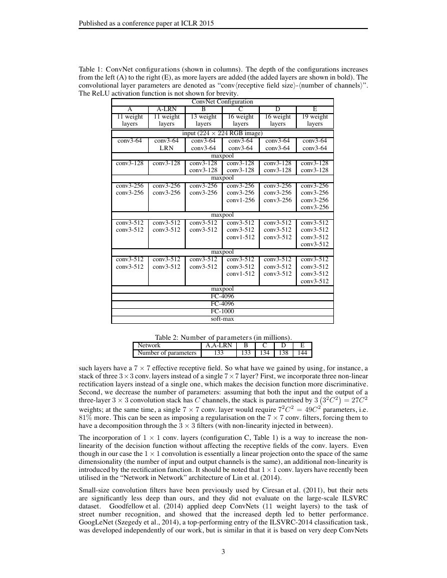2.2 CONFIGURATIONS The ConvNet conﬁgurations, evaluated in this paper, are outlined in Table 1, one per column. In the following we will refer to the nets by their names (A–E). All conﬁgurations follow the generic design presented in Sect. 2.1, and differ only in the depth: from 11 weight layers in the network A (8 conv. and 3 FC layers) to 19 weight layers in the network E (16 conv. and 3 FC layers). The width of conv. layers (the number of channels) is rather small, starting from 64 in the ﬁrst layer and then increasing by a factor of 2 after each max-pooling layer, until it reaches 512. In Table 2 we report the number of parameters for each conﬁguration. In spite of a large depth, the number of weights in our nets is not greater than the number of weights in a more shallow net with larger conv. layer widths and receptive ﬁelds (144M weights in (Sermanet et al., 2014)). 2.3 DISCUSSION Our ConvNet conﬁgurations are quite different from the ones used in the top-performing entries of the ILSVRC-2012 (Krizhevsky et al., 2012) and ILSVRC-2013 competitions (Zeiler & Fergus, 2013; Sermanet et al., 2014). Rather than using relatively large receptive ﬁelds in the ﬁrst conv. lay- ers (e.g. 11 × 11 with stride 4 in (Krizhevsky et al., 2012), or 7 × 7 with stride 2 in (Zeiler & Fergus, 2013; Sermanet et al., 2014)), we use very small 3 × 3 receptive ﬁelds throughout the whole net, which are convolved with the input at every pixel (with stride 1). It is easy to see that a stack of two 3 × 3 conv. layers (without spatial pooling in between) has an effective receptive ﬁeld of 5 × 5; three 2

Published as a conference paper at ICLR 2015 Table 1: ConvNet conﬁgurations (shown in columns). The depth of the conﬁgurations increases from the left (A) to the right (E), as more layers are added (the added layers are shown in bold). The convolutional layer parameters are denoted as “convhreceptive ﬁeld sizei-hnumber of channelsi”. The ReLU activation function is not shown for brevity. ConvNet Conﬁguration A 11 weight layers A-LRN 11 weight layers B C D E 13 weight layers 16 weight layers 16 weight layers 19 weight layers input (224 × 224 RGB image) conv3-64 conv3-64 LRN conv3-64 conv3-64 conv3-64 conv3-64 conv3-64 conv3-64 conv3-64 conv3-64 conv3-128 conv3-128 conv3-128 conv3-128 conv3-128 conv3-128 conv3-128 conv3-128 conv3-128 conv3-128 maxpool conv3-256 conv3-256 conv3-256 conv3-256 conv3-256 conv3-256 conv3-256 conv3-256 conv1-256 conv3-256 conv3-256 conv3-256 maxpool conv3-512 conv3-512 conv3-512 conv3-512 conv3-512 conv3-512 conv3-512 conv3-512 conv1-512 conv3-512 conv3-512 conv3-512 maxpool conv3-512 conv3-512 conv3-512 conv3-512 conv3-512 conv3-512 conv3-512 conv3-512 conv1-512 conv3-512 conv3-512 conv3-512 maxpool conv3-256 conv3-256 conv3-256 conv3-256 conv3-512 conv3-512 conv3-512 conv3-512 conv3-512 conv3-512 conv3-512 conv3-512 maxpool FC-4096 FC-4096 FC-1000 soft-max Table 2: Number of parameters (in millions). Network Number of parameters A,A-LRN 133 B 133 C 134 D 138 E 144 such layers have a 7 × 7 effective receptive ﬁeld. So what have we gained by using, for instance, a stack of three 3 × 3 conv. layers instead of a single 7 × 7 layer? First, we incorporate three non-linear rectiﬁcation layers instead of a single one, which makes the decision function more discriminative. Second, we decrease the number of parameters: assuming that both the input and the output of a three-layer 3 × 3 convolution stack has C channels, the stack is parametrised by 3 32C 2 = 27C 2 weights; at the same time, a single 7 × 7 conv. layer would require 72C 2 = 49C 2 parameters, i.e. 81% more. This can be seen as imposing a regularisation on the 7 × 7 conv. ﬁlters, forcing them to have a decomposition through the 3 × 3 ﬁlters (with non-linearity injected in between). The incorporation of 1 × 1 conv. layers (conﬁguration C, Table 1) is a way to increase the non- linearity of the decision function without affecting the receptive ﬁelds of the conv. layers. Even though in our case the 1 × 1 convolution is essentially a linear projection onto the space of the same dimensionality (the number of input and output channels is the same), an additional non-linearity is introduced by the rectiﬁcation function. It should be noted that 1 × 1 conv. layers have recently been utilised in the “Network in Network” architecture of Lin et al. (2014). Small-size convolution ﬁlters have been previously used by Ciresan et al. (2011), but their nets are signiﬁcantly less deep than ours, and they did not evaluate on the large-scale ILSVRC dataset. Goodfellow et al. (2014) applied deep ConvNets (11 weight layers) to the task of street number recognition, and showed that the increased depth led to better performance. GoogLeNet (Szegedy et al., 2014), a top-performing entry of the ILSVRC-2014 classiﬁcation task, was developed independently of our work, but is similar in that it is based on very deep ConvNets 3

Published as a conference paper at ICLR 2015 (22 weight layers) and small convolution ﬁlters (apart from 3 × 3, they also use 1 × 1 and 5 × 5 convolutions). Their network topology is, however, more complex than ours, and the spatial reso- lution of the feature maps is reduced more aggressively in the ﬁrst layers to decrease the amount of computation. As will be shown in Sect. 4.5, our model is outperforming that of Szegedy et al. (2014) in terms of the single-network classiﬁcation accuracy. 3 CLASSIFICATION FRAMEWORK In the previous section we presented the details of our network conﬁgurations. In this section, we describe the details of classiﬁcation ConvNet training and evaluation. 3.1 TRAINING The ConvNet training procedure generally follows Krizhevsky et al. (2012) (except for sampling the input crops from multi-scale training images, as explained later). Namely, the training is carried out by optimising the multinomial logistic regression objective using mini-batch gradient descent (based on back-propagation (LeCun et al., 1989)) with momentum. The batch size was set to 256, momentum to 0.9. The training was regularised by weight decay (the L2 penalty multiplier set to 5 · 10−4) and dropout regularisation for the ﬁrst two fully-connected layers (dropout ratio set to 0.5). The learning rate was initially set to 10−2, and then decreased by a factor of 10 when the validation set accuracy stopped improving. In total, the learning rate was decreased 3 times, and the learning was stopped after 370K iterations (74 epochs). We conjecture that in spite of the larger number of parameters and the greater depth of our nets compared to (Krizhevsky et al., 2012), the nets required less epochs to converge due to (a) implicit regularisation imposed by greater depth and smaller conv. ﬁlter sizes; (b) pre-initialisation of certain layers. The initialisation of the network weights is important, since bad initialisation can stall learning due to the instability of gradient in deep nets. To circumvent this problem, we began with training the conﬁguration A (Table 1), shallow enough to be trained with random initialisation. Then, when training deeper architectures, we initialised the ﬁrst four convolutional layers and the last three fully- connected layers with the layers of net A (the intermediate layers were initialised randomly). We did not decrease the learning rate for the pre-initialised layers, allowing them to change during learning. For random initialisation (where applicable), we sampled the weights from a normal distribution with the zero mean and 10−2 variance. The biases were initialised with zero. It is worth noting that after the paper submission we found that it is possible to initialise the weights without pre-training by using the random initialisation procedure of Glorot & Bengio (2010). To obtain the ﬁxed-size 224×224 ConvNet input images, they were randomly cropped from rescaled training images (one crop per image per SGD iteration). To further augment the training set, the crops underwent random horizontal ﬂipping and random RGB colour shift (Krizhevsky et al., 2012). Training image rescaling is explained below. Training image size. Let S be the smallest side of an isotropically-rescaled training image, from which the ConvNet input is cropped (we also refer to S as the training scale). While the crop size is ﬁxed to 224 × 224, in principle S can take on any value not less than 224: for S = 224 the crop will capture whole-image statistics, completely spanning the smallest side of a training image; for S ≫ 224 the crop will correspond to a small part of the image, containing a small object or an object part. We consider two approaches for setting the training scale S. The ﬁrst is to ﬁx S, which corresponds to single-scale training (note that image content within the sampled crops can still represent multi- scale image statistics). In our experiments, we evaluated models trained at two ﬁxed scales: S = 256 (which has been widely used in the prior art (Krizhevsky et al., 2012; Zeiler & Fergus, 2013; Sermanet et al., 2014)) and S = 384. Given a ConvNet conﬁguration, we ﬁrst trained the network using S = 256. To speed-up training of the S = 384 network, it was initialised with the weights pre-trained with S = 256, and we used a smaller initial learning rate of 10−3. The second approach to setting S is multi-scale training, where each training image is individually rescaled by randomly sampling S from a certain range [Smin, Smax] (we used Smin = 256 and Smax = 512). Since objects in images can be of different size, it is beneﬁcial to take this into account during training. This can also be seen as training set augmentation by scale jittering, where a single 4

Published as a conference paper at ICLR 2015 model is trained to recognise objects over a wide range of scales. For speed reasons, we trained multi-scale models by ﬁne-tuning all layers of a single-scale model with the same conﬁguration, pre-trained with ﬁxed S = 384. 3.2 TESTING At test time, given a trained ConvNet and an input image, it is classiﬁed in the following way. First, it is isotropically rescaled to a pre-deﬁned smallest image side, denoted as Q (we also refer to it as the test scale). We note that Q is not necessarily equal to the training scale S (as we will show in Sect. 4, using several values of Q for each S leads to improved performance). Then, the network is applied densely over the rescaled test image in a way similar to (Sermanet et al., 2014). Namely, the fully-connected layers are ﬁrst converted to convolutional layers (the ﬁrst FC layer to a 7 × 7 conv. layer, the last two FC layers to 1 × 1 conv. layers). The resulting fully-convolutional net is then applied to the whole (uncropped) image. The result is a class score map with the number of channels equal to the number of classes, and a variable spatial resolution, dependent on the input image size. Finally, to obtain a ﬁxed-size vector of class scores for the image, the class score map is spatially averaged (sum-pooled). We also augment the test set by horizontal ﬂipping of the images; the soft-max class posteriors of the original and ﬂipped images are averaged to obtain the ﬁnal scores for the image. Since the fully-convolutional network is applied over the whole image, there is no need to sample multiple crops at test time (Krizhevsky et al., 2012), which is less efﬁcient as it requires network re-computation for each crop. At the same time, using a large set of crops, as done by Szegedy et al. (2014), can lead to improved accuracy, as it results in a ﬁner sampling of the input image compared to the fully-convolutional net. Also, multi-crop evaluation is complementary to dense evaluation due to different convolution boundary conditions: when applying a ConvNet to a crop, the convolved feature maps are padded with zeros, while in the case of dense evaluation the padding for the same crop naturally comes from the neighbouring parts of an image (due to both the convolutions and spatial pooling), which substantially increases the overall network receptive ﬁeld, so more context is captured. While we believe that in practice the increased computation time of multiple crops does not justify the potential gains in accuracy, for reference we also evaluate our networks using 50 crops per scale (5 × 5 regular grid with 2 ﬂips), for a total of 150 crops over 3 scales, which is comparable to 144 crops over 4 scales used by Szegedy et al. (2014). 3.3 IMPLEMENTATION DETAILS Our implementation is derived from the publicly available C++ Caffe toolbox (Jia, 2013) (branched out in December 2013), but contains a number of signiﬁcant modiﬁcations, allowing us to perform training and evaluation on multiple GPUs installed in a single system, as well as train and evaluate on full-size (uncropped) images at multiple scales (as described above). Multi-GPU training exploits data parallelism, and is carried out by splitting each batch of training images into several GPU batches, processed in parallel on each GPU. After the GPU batch gradients are computed, they are averaged to obtain the gradient of the full batch. Gradient computation is synchronous across the GPUs, so the result is exactly the same as when training on a single GPU. While more sophisticated methods of speeding up ConvNet training have been recently pro- posed (Krizhevsky, 2014), which employ model and data parallelism for different layers of the net, we have found that our conceptually much simpler scheme already provides a speedup of 3.75 times on an off-the-shelf 4-GPU system, as compared to using a single GPU. On a system equipped with four NVIDIA Titan Black GPUs, training a single net took 2–3 weeks depending on the architecture. 4 CLASSIFICATION EXPERIMENTS Dataset. In this section, we present the image classiﬁcation results achieved by the described ConvNet architectures on the ILSVRC-2012 dataset (which was used for ILSVRC 2012–2014 chal- lenges). The dataset includes images of 1000 classes, and is split into three sets: training (1.3M images), validation (50K images), and testing (100K images with held-out class labels). The clas- siﬁcation performance is evaluated using two measures: the top-1 and top-5 error. The former is a multi-class classiﬁcation error, i.e. the proportion of incorrectly classiﬁed images; the latter is the 5

Published as a conference paper at ICLR 2015 main evaluation criterion used in ILSVRC, and is computed as the proportion of images such that the ground-truth category is outside the top-5 predicted categories. For the majority of experiments, we used the validation set as the test set. Certain experiments were also carried out on the test set and submitted to the ofﬁcial ILSVRC server as a “VGG” team entry to the ILSVRC-2014 competition (Russakovsky et al., 2014). 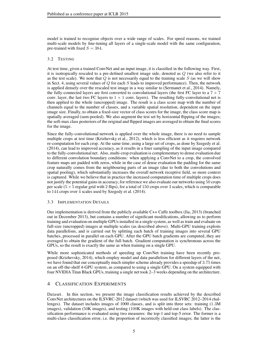4.1 SINGLE SCALE EVALUATION We begin with evaluating the performance of individual ConvNet models at a single scale with the layer conﬁgurations described in Sect. 2.2. The test image size was set as follows: Q = S for ﬁxed S, and Q = 0.5(Smin + Smax) for jittered S ∈ [Smin, Smax]. The results of are shown in Table 3. First, we note that using local response normalisation (A-LRN network) does not improve on the model A without any normalisation layers. We thus do not employ normalisation in the deeper architectures (B–E). Second, we observe that the classiﬁcation error decreases with the increased ConvNet depth: from 11 layers in A to 19 layers in E. Notably, in spite of the same depth, the conﬁguration C (which contains three 1 × 1 conv. layers), performs worse than the conﬁguration D, which uses 3 × 3 conv. layers throughout the network. This indicates that while the additional non-linearity does help (C is better than B), it is also important to capture spatial context by using conv. ﬁlters with non-trivial receptive ﬁelds (D is better than C). The error rate of our architecture saturates when the depth reaches 19 layers, but even deeper models might be beneﬁcial for larger datasets. We also compared the net B with a shallow net with ﬁve 5 × 5 conv. layers, which was derived from B by replacing each pair of 3 × 3 conv. layers with a single 5 × 5 conv. layer (which has the same receptive ﬁeld as explained in Sect. 2.3). The top-1 error of the shallow net was measured to be 7% higher than that of B (on a center crop), which conﬁrms that a deep net with small ﬁlters outperforms a shallow net with larger ﬁlters. Finally, scale jittering at training time (S ∈ [256; 512]) leads to signiﬁcantly better results than training on images with ﬁxed smallest side (S = 256 or S = 384), even though a single scale is used at test time. This conﬁrms that training set augmentation by scale jittering is indeed helpful for capturing multi-scale image statistics. Table 3: ConvNet performance at a single test scale. ConvNet conﬁg. (Table 1) smallest image side train (S) test (Q) top-1 val. error (%) top-5 val. 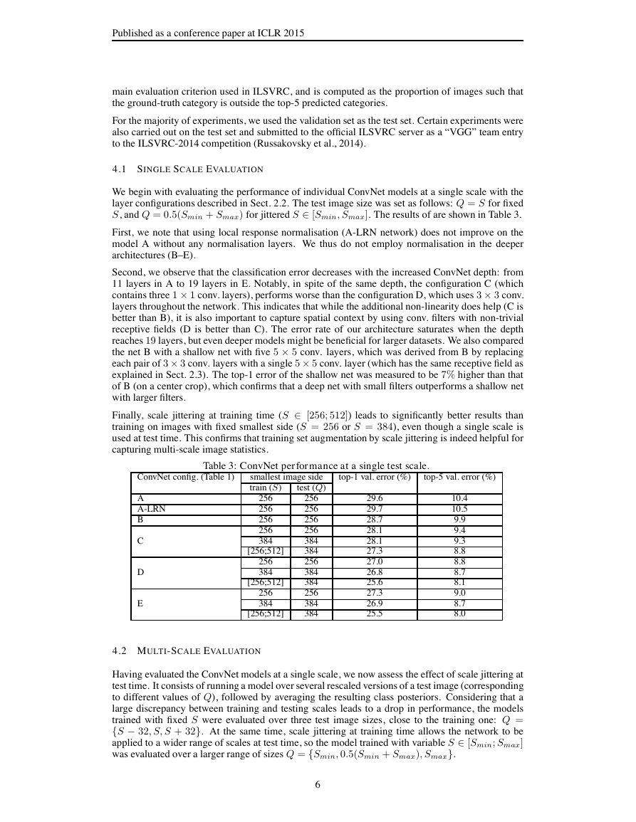error (%) A A-LRN B C D E 256 256 256 256 384 [256;512] 256 384 [256;512] 256 384 [256;512] 256 256 256 256 384 384 256 384 384 256 384 384 29.6 29.7 28.7 28.1 28.1 27.3 27.0 26.8 25.6 27.3 26.9 25.5 10.4 10.5 9.9 9.4 9.3 8.8 8.8 8.7 8.1 9.0 8.7 8.0 4.2 MULTI-SCALE EVALUATION Having evaluated the ConvNet models at a single scale, we now assess the effect of scale jittering at test time. It consists of running a model over several rescaled versions of a test image (corresponding to different values of Q), followed by averaging the resulting class posteriors. Considering that a large discrepancy between training and testing scales leads to a drop in performance, the models trained with ﬁxed S were evaluated over three test image sizes, close to the training one: Q = {S − 32, S, S + 32}. At the same time, scale jittering at training time allows the network to be applied to a wider range of scales at test time, so the model trained with variable S ∈ [Smin; Smax] was evaluated over a larger range of sizes Q = {Smin, 0.5(Smin + Smax), Smax}. 6

Published as a conference paper at ICLR 2015 The results, presented in Table 4, indicate that scale jittering at test time leads to better performance (as compared to evaluating the same model at a single scale, shown in Table 3). As before, the deepest conﬁgurations (D and E) perform the best, and scale jittering is better than training with a ﬁxed smallest side S. Our best single-network performance on the validation set is 24.8%/7.5% top-1/top-5 error (highlighted in bold in Table 4). On the test set, the conﬁguration E achieves 7.3% top-5 error. Table 4: ConvNet performance at multiple test scales. ConvNet conﬁg. (Table 1) smallest image side test (Q) train (S) top-1 val. error (%) top-5 val. 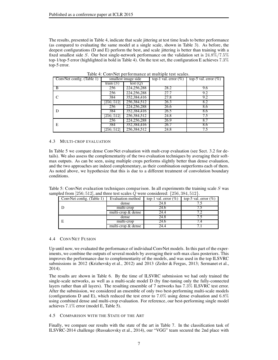error (%) B C D E 256 256 384 [256; 512] 256 384 [256; 512] 256 384 [256; 512] 224,256,288 224,256,288 352,384,416 256,384,512 224,256,288 352,384,416 256,384,512 224,256,288 352,384,416 256,384,512 28.2 27.7 27.8 26.3 26.6 26.5 24.8 26.9 26.7 24.8 9.6 9.2 9.2 8.2 8.6 8.6 7.5 8.7 8.6 7.5 4.3 MULTI-CROP EVALUATION In Table 5 we compare dense ConvNet evaluation with mult-crop evaluation (see Sect. 3.2 for de- tails). We also assess the complementarity of the two evaluation techniques by averaging their soft- max outputs. As can be seen, using multiple crops performs slightly better than dense evaluation, and the two approaches are indeed complementary, as their combination outperforms each of them. As noted above, we hypothesize that this is due to a different treatment of convolution boundary conditions. Table 5: ConvNet evaluation techniques comparison. In all experiments the training scale S was sampled from [256; 512], and three test scales Q were considered: {256, 384, 512}. ConvNet conﬁg. (Table 1) Evaluation method top-1 val. error (%) top-5 val. error (%) D E 4.4 CONVNET FUSION dense multi-crop multi-crop & dense dense multi-crop multi-crop & dense 24.8 24.6 24.4 24.8 24.6 24.4 7.5 7.5 7.2 7.5 7.4 7.1 Up until now, we evaluated the performance of individual ConvNet models. In this part of the exper- iments, we combine the outputs of several models by averaging their soft-max class posteriors. This improves the performance due to complementarity of the models, and was used in the top ILSVRC submissions in 2012 (Krizhevsky et al., 2012) and 2013 (Zeiler & Fergus, 2013; Sermanet et al., 2014). 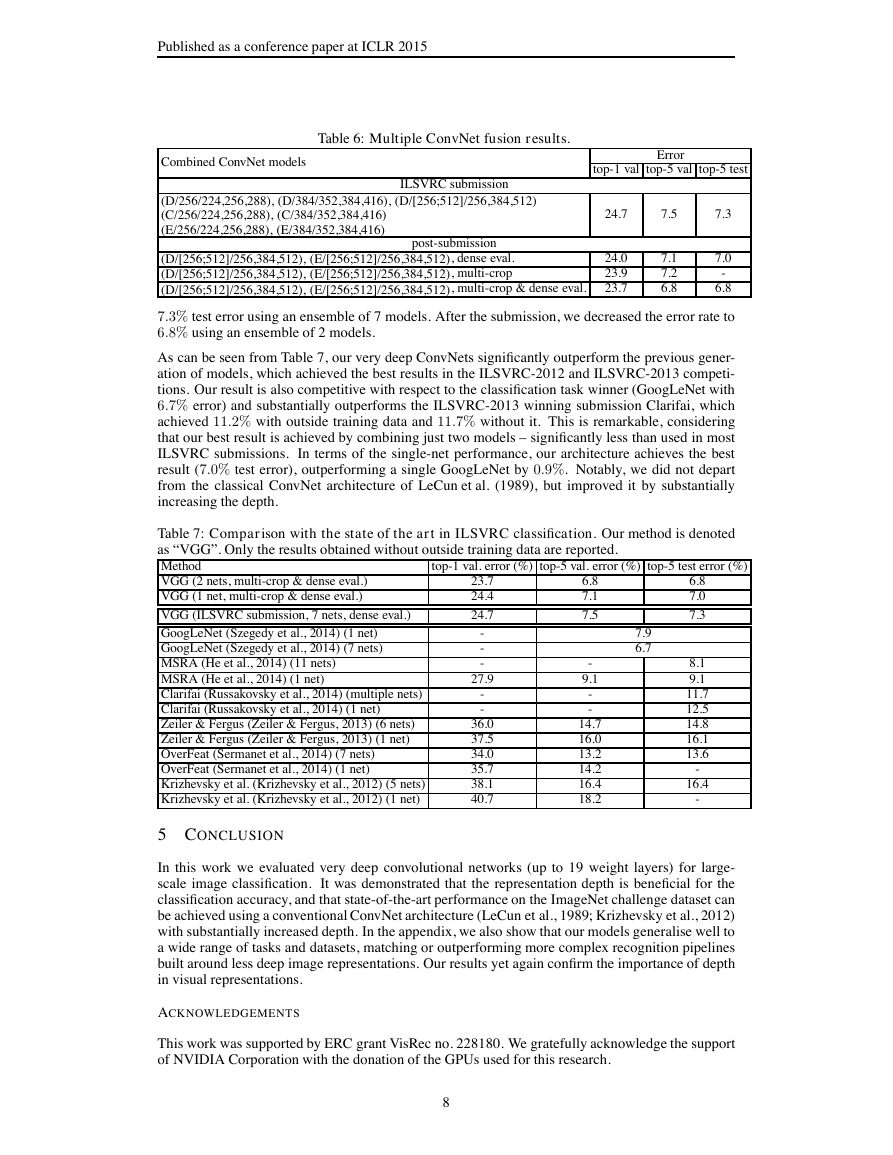The results are shown in Table 6. By the time of ILSVRC submission we had only trained the single-scale networks, as well as a multi-scale model D (by ﬁne-tuning only the fully-connected layers rather than all layers). The resulting ensemble of 7 networks has 7.3% ILSVRC test error. After the submission, we considered an ensemble of only two best-performing multi-scale models (conﬁgurations D and E), which reduced the test error to 7.0% using dense evaluation and 6.8% using combined dense and multi-crop evaluation. For reference, our best-performing single model achieves 7.1% error (model E, Table 5). 4.5 COMPARISON WITH THE STATE OF THE ART Finally, we compare our results with the state of the art in Table 7. In the classiﬁcation task of ILSVRC-2014 challenge (Russakovsky et al., 2014), our “VGG” team secured the 2nd place with 7

Published as a conference paper at ICLR 2015 Combined ConvNet models Table 6: Multiple ConvNet fusion results. Error top-1 val top-5 val top-5 test ILSVRC submission (D/256/224,256,288), (D/384/352,384,416), (D/[256;512]/256,384,512) (C/256/224,256,288), (C/384/352,384,416) (E/256/224,256,288), (E/384/352,384,416) post-submission (D/[256;512]/256,384,512), (E/[256;512]/256,384,512), dense eval. (D/[256;512]/256,384,512), (E/[256;512]/256,384,512), multi-crop (D/[256;512]/256,384,512), (E/[256;512]/256,384,512), multi-crop & dense eval. 24.7 24.0 23.9 23.7 7.5 7.1 7.2 6.8 7.3 7.0 - 6.8 7.3% test error using an ensemble of 7 models. After the submission, we decreased the error rate to 6.8% using an ensemble of 2 models. As can be seen from Table 7, our very deep ConvNets signiﬁcantly outperform the previous gener- ation of models, which achieved the best results in the ILSVRC-2012 and ILSVRC-2013 competi- tions. Our result is also competitive with respect to the classiﬁcation task winner (GoogLeNet with 6.7% error) and substantially outperforms the ILSVRC-2013 winning submission Clarifai, which achieved 11.2% with outside training data and 11.7% without it. This is remarkable, considering that our best result is achieved by combining just two models – signiﬁcantly less than used in most ILSVRC submissions. In terms of the single-net performance, our architecture achieves the best result (7.0% test error), outperforming a single GoogLeNet by 0.9%. Notably, we did not depart from the classical ConvNet architecture of LeCun et al. (1989), but improved it by substantially increasing the depth. top-1 val. error (%) top-5 val. error (%) top-5 test error (%) 23.7 24.4 24.7 Table 7: Comparison with the state of the art in ILSVRC classiﬁcation. Our method is denoted as “VGG”. Only the results obtained without outside training data are reported. Method VGG (2 nets, multi-crop & dense eval.) VGG (1 net, multi-crop & dense eval.) VGG (ILSVRC submission, 7 nets, dense eval.) GoogLeNet (Szegedy et al., 2014) (1 net) GoogLeNet (Szegedy et al., 2014) (7 nets) MSRA (He et al., 2014) (11 nets) MSRA (He et al., 2014) (1 net) Clarifai (Russakovsky et al., 2014) (multiple nets) Clarifai (Russakovsky et al., 2014) (1 net) Zeiler & Fergus (Zeiler & Fergus, 2013) (6 nets) Zeiler & Fergus (Zeiler & Fergus, 2013) (1 net) OverFeat (Sermanet et al., 2014) (7 nets) OverFeat (Sermanet et al., 2014) (1 net) Krizhevsky et al. (Krizhevsky et al., 2012) (5 nets) Krizhevsky et al. (Krizhevsky et al., 2012) (1 net) 8.1 9.1 11.7 12.5 14.8 16.1 13.6 36.0 37.5 34.0 35.7 38.1 40.7 14.7 16.0 13.2 14.2 16.4 18.2 6.8 7.1 7.5 - 9.1 - - - - - - - 27.9 7.9 6.7 6.8 7.0 7.3 16.4 - - 5 CONCLUSION In this work we evaluated very deep convolutional networks (up to 19 weight layers) for large- scale image classiﬁcation. It was demonstrated that the representation depth is beneﬁcial for the classiﬁcation accuracy, and that state-of-the-art performance on the ImageNet challenge dataset can be achieved using a conventional ConvNet architecture (LeCun et al., 1989; Krizhevsky et al., 2012) with substantially increased depth. In the appendix, we also show that our models generalise well to a wide range of tasks and datasets, matching or outperforming more complex recognition pipelines built around less deep image representations. Our results yet again conﬁrm the importance of depth in visual representations. ACKNOWLEDGEMENTS This work was supported by ERC grant VisRec no. 228180. We gratefully acknowledge the support of NVIDIA Corporation with the donation of the GPUs used for this research. 8

分享到：

赞收藏

资料库

【5】Very deep convolutional networks for large-scale image recogn....pdf

相关推荐

人工智能

热门标签

最新资料