RCWA一维代码.pdf-资料库

rcwareader-11052521-16359647431339776123.pdf-第1页.png

第1页 / 共13页

rcwareader-11052521-16359647431339776123.pdf-第2页.png

第2页 / 共13页

rcwareader-11052521-16359647431339776123.pdf-第3页.png

第3页 / 共13页

rcwareader-11052521-16359647431339776123.pdf-第4页.png

第4页 / 共13页

rcwareader-11052521-16359647431339776123.pdf-第5页.png

第5页 / 共13页

rcwareader-11052521-16359647431339776123.pdf-第6页.png

第6页 / 共13页

rcwareader-11052521-16359647431339776123.pdf-第7页.png

第7页 / 共13页

rcwareader-11052521-16359647431339776123.pdf-第8页.png

第8页 / 共13页

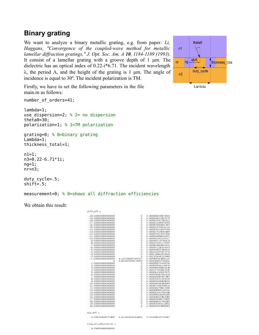
Binary grating We want to analyze a binary metallic grating, e.g. from paper: Li, Haggans, "Convergence of the coupled-wave method for metallic lamellar diffraction gratings," J. Opt. Soc. Am. A 10, 1184-1189 (1993). It consist of a lamellar grating with a groove depth of 1 μm. The dielectric has an optical index of 0.22-i*6.71. The incident wavelength λ, the period Λ, and the height of the grating is 1 μm. The angle of incidence is equal to 30º. The incident polarization is TM. 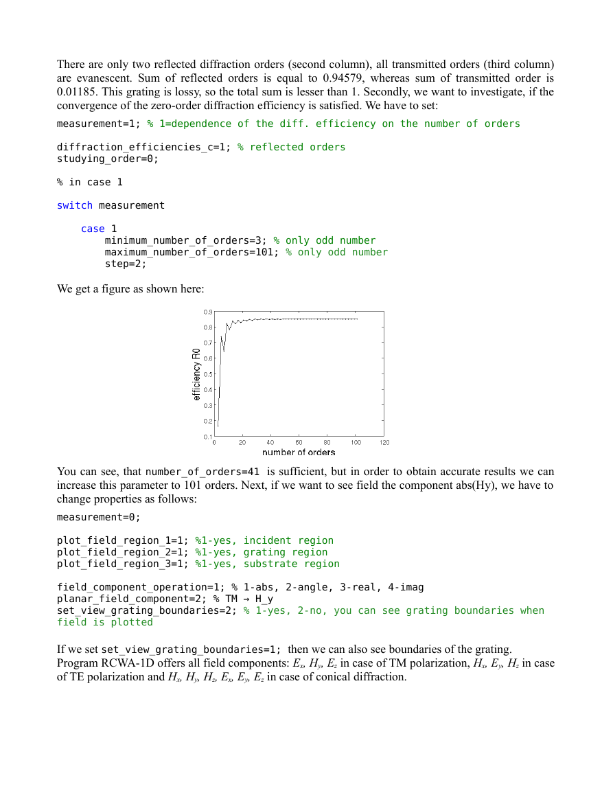Firstly, we have to set the following parameters in the file main.m as follows: number_of_orders=41; lambda=1; use_dispersion=2; % 2= no dispersion theta0=30; polarization=1; % 1=TM polarization grating=0; % 0=binary grating Lambda=1; thickness_total=1; n1=1; n3=0.22-6.71*1i; ng=1; nr=n3; duty_cycle=.5; shift=.5; measurement=0; % 0=shows all diffraction efficiencies We obtain this result:

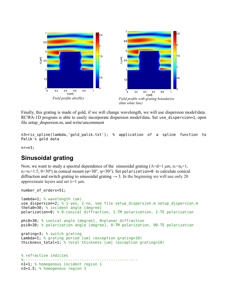
There are only two reflected diffraction orders (second column), all transmitted orders (third column) are evanescent. Sum of reflected orders is equal to 0.94579, whereas sum of transmitted order is 0.01185. This grating is lossy, so the total sum is lesser than 1. Secondly, we want to investigate, if the convergence of the zero-order diffraction efficiency is satisfied. We have to set: measurement=1; % 1=dependence of the diff. efficiency on the number of orders diffraction_efficiencies_c=1; % reflected orders studying_order=0; % in case 1 switch measurement case 1 minimum_number_of_orders=3; % only odd number maximum_number_of_orders=101; % only odd number step=2; We get a figure as shown here: You can see, that number_of_orders=41 is sufficient, but in order to obtain accurate results we can increase this parameter to 101 orders. Next, if we want to see field the component abs(Hy), we have to change properties as follows: measurement=0; plot_field_region_1=1; %1-yes, incident region plot_field_region_2=1; %1-yes, grating region plot_field_region_3=1; %1-yes, substrate region field_component_operation=1; % 1-abs, 2-angle, 3-real, 4-imag planar_field_component=2; % TM → H_y set_view_grating_boundaries=2; % 1-yes, 2-no, you can see grating boundaries when field is plotted If we set set_view_grating_boundaries=1; then we can also see boundaries of the grating. Program RCWA-1D offers all field components: Ex, Hy, Ez in case of TM polarization, Hx, Ey, Hz in case of TE polarization and Hx, Hy, Hz, Ex, Ey, Ez in case of conical diffraction.

Field profile abs(Hy) Field profile with grating boundaries (thin white line) Finally, this grating is made of gold, if we will change wavelength, we will use dispersion model/data. RCWA-1D program is able to easily incorporate dispersion model/data. Set use_dispersion=1, open file setup_dispersion.m, and write/uncomment n3=rix_spline(lambda,'gold_palik.txt'); % application of a spline function to Palik's gold data nr=n3; Sinusoidal grating Now, we want to study a spectral dependence of the sinusoidal grating (Λ=d=1 μm, n1=ng=1, n3=nr=1.5, θ=30º) in conical mount (φ=30°, ψ=30°). Set polarization=0 to calculate conical diffraction and switch grating to sinusoidal grating → 3. In the beginning we will use only 20 approximate layers and set λ=1 μm. number_of_orders=51; lambda=1; % wavelength (um) use_dispersion=2; % 1-yes, 2-no, see file setup_dispersion.m setup_dispersion.m theta0=30; % incident angle [degree] polarization=0; % 0-conical diffraction, 1-TM polarization, 2-TE polarization phi0=30; % conical angle [degree], 0=planar diffraction psi0=30; % polarization angle [degree], 0-TM polarization, 90-TE polarization grating=3; % switch grating Lambda=1; % grating period [um] (exception grating=10) thickness_total=1; % total thickness [um] (exception grating=10) % refractive indicies %--------------------------------------------------- n1=1; % homogenous incident region 1 n3=1.5; % homogenous region 3

ng=1; % Groove indicies nr=n3; % Ridge indices switch grating case 3 % sinusoidal grating number_of_layers=20; measurement=0; We get this result: -3.000000000000000 0 0.013089017931952 -2.000000000000000 0.004421523159508 0.024058203757450 -1.000000000000000 0.004224700988475 0.278806883502640 0 0.000676667854081 0.143246725101695 1.000000000000000 0.005561992124616 0.513569971548332 2.000000000000000 0 0.012344314163998 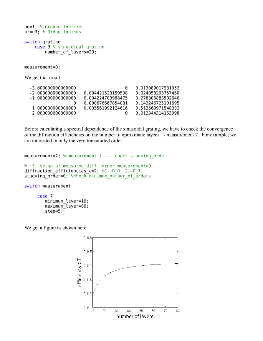Before calculating a spectral dependence of the sinusoidal grating, we have to check the convergence of the diffraction efficiencies on the number of aproximate layers → measurement 7. For example, we are interested in only the zero transmitted order. measurement=7; % measurement 1 --- check studying_order % !!! setup of measured diff. order measurement>0 diffraction_efficiencies_c=2; %1--D_R, 2--D_T studying_order=0; %check minimum_number_of_orders switch measurement case 7 minimum_layer=10; maximum_layer=80; step=5; We get a figure as shown here.

You can see in the figure above that we should increase the number of layers, i.e. to 50 layers. To study spectral dependence (0.7—1.3 μm) set measurement to 2. To save all results of all diffraction orders set save_m to 1 and choose a proper name of this file. 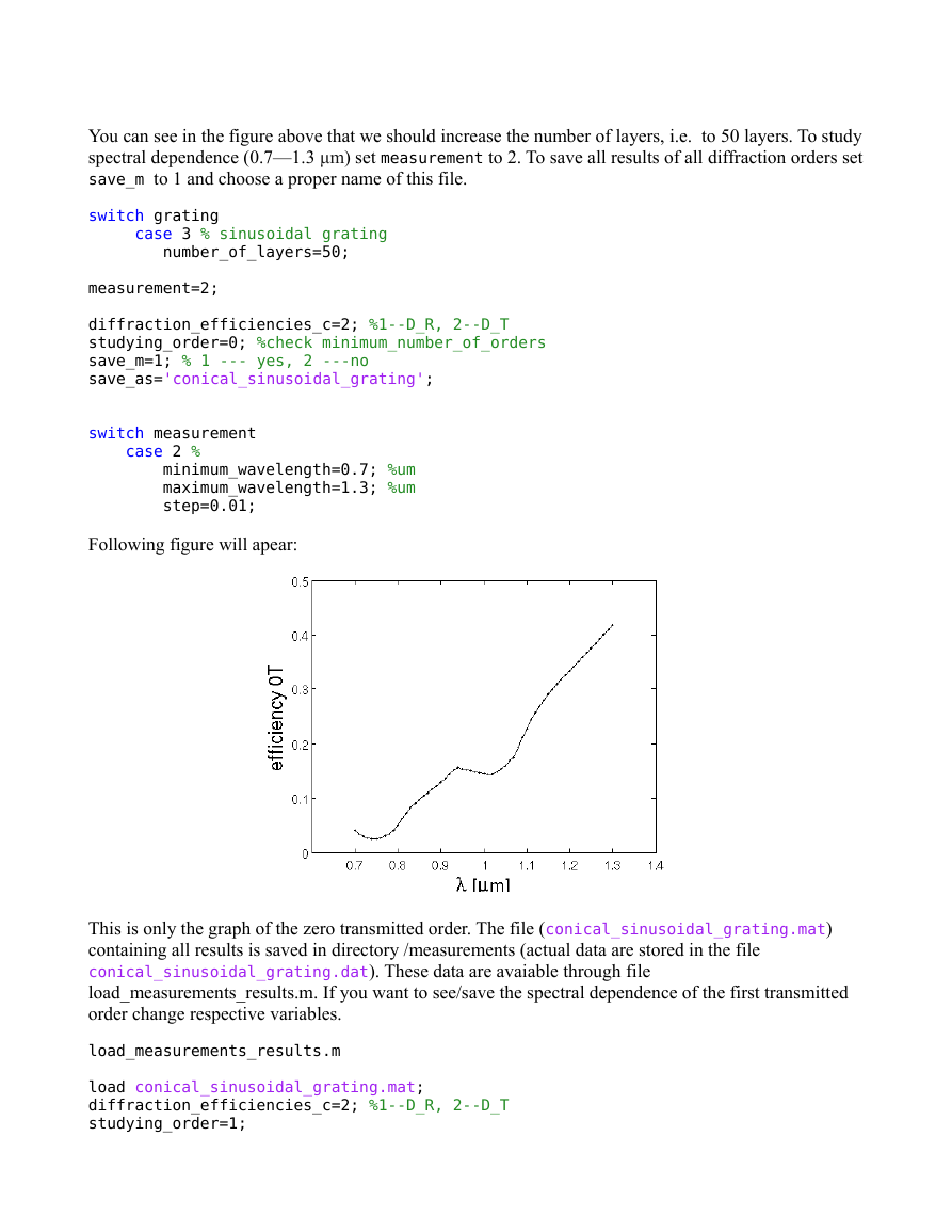switch grating case 3 % sinusoidal grating number_of_layers=50; measurement=2; diffraction_efficiencies_c=2; %1--D_R, 2--D_T studying_order=0; %check minimum_number_of_orders save_m=1; % 1 --- yes, 2 ---no save_as='conical_sinusoidal_grating'; switch measurement case 2 % minimum_wavelength=0.7; %um maximum_wavelength=1.3; %um step=0.01; Following figure will apear: This is only the graph of the zero transmitted order. The file (conical_sinusoidal_grating.mat) containing all results is saved in directory /measurements (actual data are stored in the file conical_sinusoidal_grating.dat). 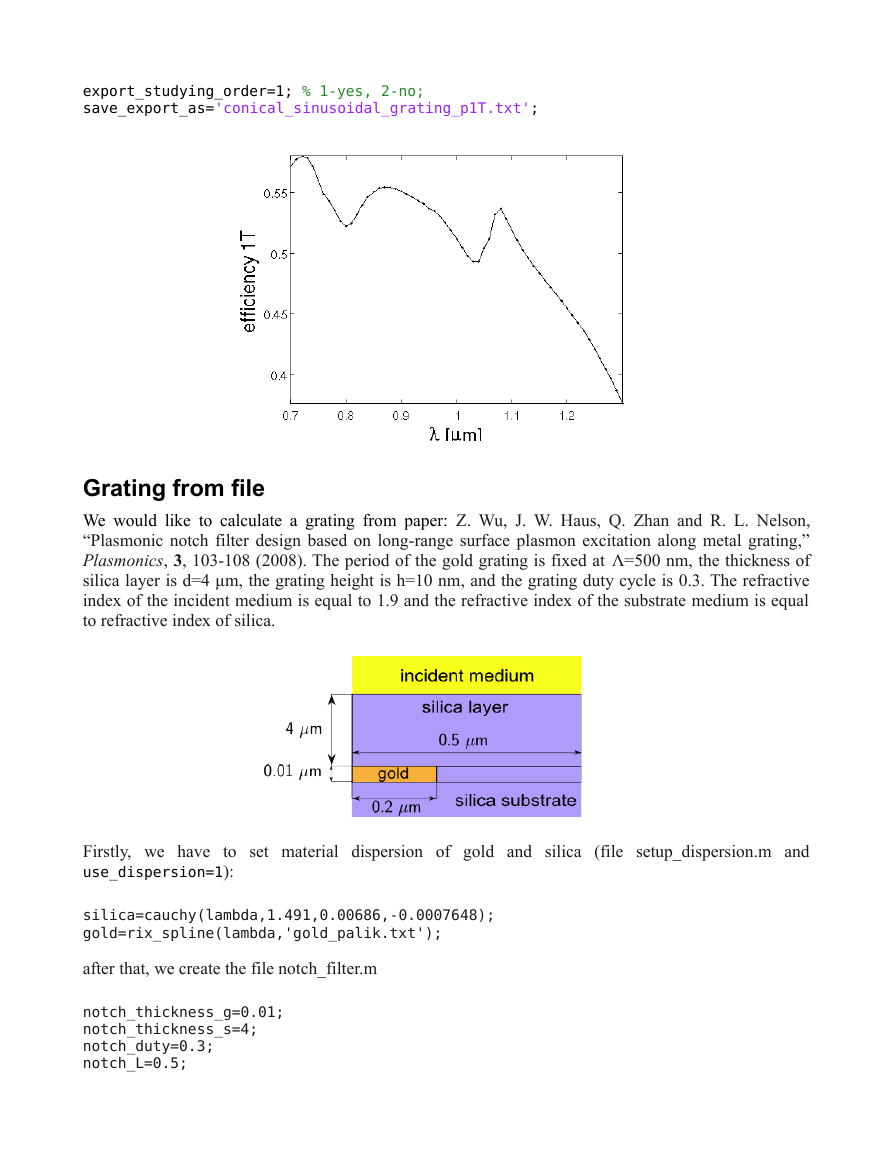These data are avaiable through file load_measurements_results.m. If you want to see/save the spectral dependence of the first transmitted order change respective variables. load_measurements_results.m load conical_sinusoidal_grating.mat; diffraction_efficiencies_c=2; %1--D_R, 2--D_T studying_order=1;

export_studying_order=1; % 1-yes, 2-no; save_export_as='conical_sinusoidal_grating_p1T.txt'; Grating from file We would like to calculate a grating from paper: Z. Wu, J. W. Haus, Q. Zhan and R. L. Nelson, “Plasmonic notch filter design based on long-range surface plasmon excitation along metal grating,” Plasmonics, 3, 103-108 (2008). The period of the gold grating is fixed at Λ=500 nm, the thickness of silica layer is d=4 μm, the grating height is h=10 nm, and the grating duty cycle is 0.3. The refractive index of the incident medium is equal to 1.9 and the refractive index of the substrate medium is equal to refractive index of silica. Firstly, we have to set material dispersion of gold and silica (file setup_dispersion.m and use_dispersion=1): silica=cauchy(lambda,1.491,0.00686,-0.0007648); gold=rix_spline(lambda,'gold_palik.txt'); after that, we create the file notch_filter.m notch_thickness_g=0.01; notch_thickness_s=4; notch_duty=0.3; notch_L=0.5;

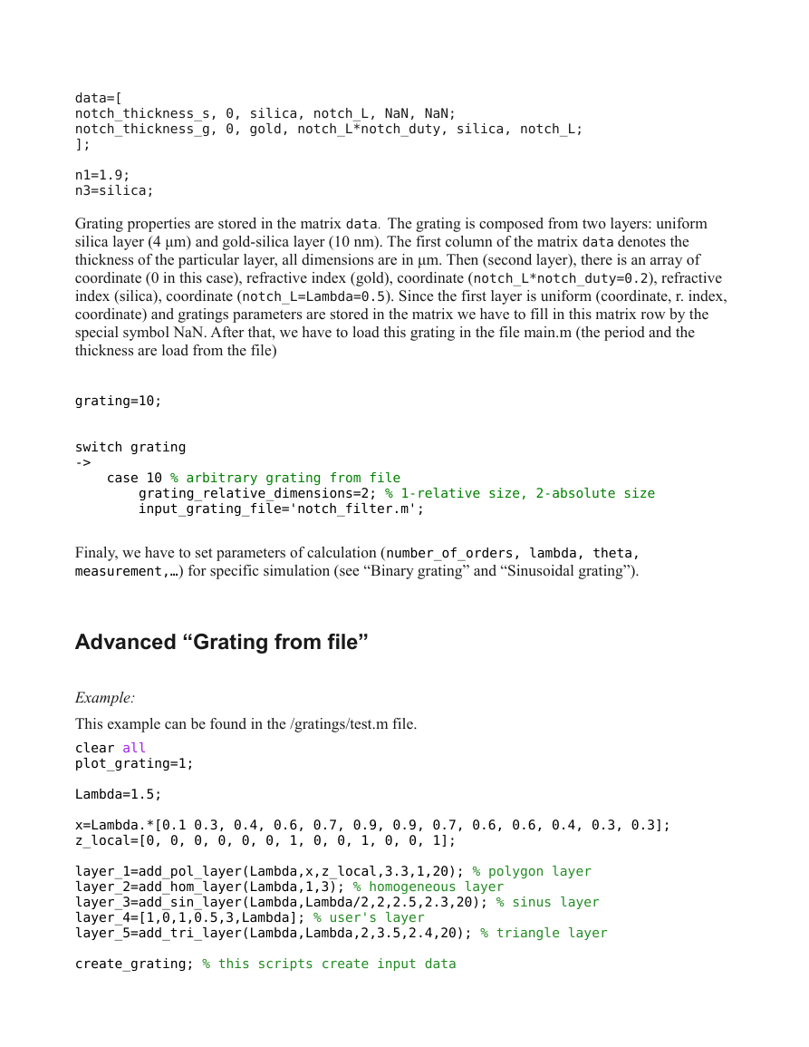
data=[ notch_thickness_s, 0, silica, notch_L, NaN, NaN; notch_thickness_g, 0, gold, notch_L*notch_duty, silica, notch_L; ]; n1=1.9; n3=silica; Grating properties are stored in the matrix data. The grating is composed from two layers: uniform silica layer (4 μm) and gold-silica layer (10 nm). The first column of the matrix data denotes the thickness of the particular layer, all dimensions are in μm. Then (second layer), there is an array of coordinate (0 in this case), refractive index (gold), coordinate (notch_L*notch_duty=0.2), refractive index (silica), coordinate (notch_L=Lambda=0.5). Since the first layer is uniform (coordinate, r. index, coordinate) and gratings parameters are stored in the matrix we have to fill in this matrix row by the special symbol NaN. After that, we have to load this grating in the file main.m (the period and the thickness are load from the file) grating=10; switch grating -> case 10 % arbitrary grating from file grating_relative_dimensions=2; % 1-relative size, 2-absolute size input_grating_file='notch_filter.m'; Finaly, we have to set parameters of calculation (number_of_orders, lambda, theta, measurement,…) for specific simulation (see “Binary grating” and “Sinusoidal grating”). 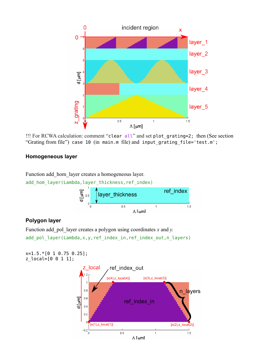Advanced “Grating from file” Example: This example can be found in the /gratings/test.m file. clear all plot_grating=1; Lambda=1.5; x=Lambda.*[0.1 0.3, 0.4, 0.6, 0.7, 0.9, 0.9, 0.7, 0.6, 0.6, 0.4, 0.3, 0.3]; z_local=[0, 0, 0, 0, 0, 0, 1, 0, 0, 1, 0, 0, 1]; layer_1=add_pol_layer(Lambda,x,z_local,3.3,1,20); % polygon layer layer_2=add_hom_layer(Lambda,1,3); % homogeneous layer layer_3=add_sin_layer(Lambda,Lambda/2,2,2.5,2.3,20); % sinus layer layer_4=[1,0,1,0.5,3,Lambda]; % user's layer layer_5=add_tri_layer(Lambda,Lambda,2,3.5,2.4,20); % triangle layer create_grating; % this scripts create input data

!!! For RCWA calculation: comment “clear all” and set plot_grating=2; then (See section “Grating from file”) case 10 (in main.m file) and input_grating_file='test.m'; Homogeneous layer Function add_hom_layer creates a homogeneous layer. add_hom_layer(Lambda,layer_thickness,ref_index) Polygon layer Function add_pol_layer creates a polygon using coordinates x and y. add_pol_layer(Lambda,x,y,ref_index_in,ref_index_out,n_layers) x=1.5.*[0 1 0.75 0.25]; z_local=[0 0 1 1];

资料库

RCWA一维代码.pdf

相关推荐

信息化

热门标签

最新资料