Learning Multi-scale Block Local Binary
Patterns for Face Recognition
Shengcai Liao, Xiangxin Zhu, Zhen Lei, Lun Zhang, and Stan Z. Li
Center for Biometrics and Security Research &
National Laboratory of Pattern Recognition,
Institute of Automation, Chinese Academy of Sciences,
95 Zhongguancun Donglu, Beijing 100080, China
{scliao,xxzhu,zlei,lzhang,szli}@nlpr.ia.ac.cn
http://www.cbsr.ia.ac.cn
Abstract. In this paper, we propose a novel representation, called Multi-
scale Block Local Binary Pattern (MB-LBP), and apply it to face recogni-
tion. The Local Binary Pattern (LBP) has been proved to be effective for
image representation, but it is too local to be robust. In MB-LBP, the com-
putation is done based on average values of block subregions, instead of
individual pixels. In this way, MB-LBP code presents several advantages:
(1) It is more robust than LBP; (2) it encodes not only microstructures but
also macrostructures of image patterns, and hence provides a more com-
plete image representation than the basic LBP operator; and (3) MB-LBP
can be computed very efficiently using integral images. Furthermore, in or-
der to reflect the uniform appearance of MB-LBP, we redefine the uniform
patterns via statistical analysis. Finally, AdaBoost learning is applied to
select most effective uniform MB-LBP features and construct face classi-
fiers. Experiments on Face Recognition Grand Challenge (FRGC) ver2.0
database show that the proposed MB-LBP method significantly outper-
forms other LBP based face recognition algorithms.
Keywords: LBP, MB-LBP, Face Recognition, AdaBoost.
1 Introduction
Face recognition from images has been a hot research topic in computer vision
for recent two decades. This is because face recognition has potential applica-
tion values as well as theoretical challenges. Many appearance-based approaches
have been proposed to deal with face recognition problems. Holistic subspace
approach, such as PCA [14] and LDA [3] based methods, has significantly ad-
vanced face recognition techniques. Using PCA, a face subspace is constructed
to represent “optimally” only the face; using LDA, a discriminant subspace is
constructed to distinguish “optimally” faces of different persons. Another ap-
proach is to construct a local appearance-based feature space, using appropriate
image filters, so the distributions of faces are less affected by various changes. Lo-
cal features analysis (LFA) [10], Gabor wavelet-based features [16,6] are among
these.
S.-W. Lee and S.Z. Li (Eds.): ICB 2007, LNCS 4642, pp. 828–837, 2007.
c Springer-Verlag Berlin Heidelberg 2007
�
Learning MB-LBP for Face Recognition
829
Recently, Local Binary Patterns (LBP) is introduced as a powerful local de-
scriptor for microstructures of images [8]. The LBP operator labels the pixels of
an image by thresholding the 3 × 3-neighborhood of each pixel with the center
value and considering the result as a binary string or a decimal number. Recently,
Ahonen et al proposed a novel approach for face recognition, which takes advan-
tage of the Local Binary Pattern (LBP) histogram [1]. In their method, the face
image is equally divided into small sub-windows from which the LBP features
are extracted and concatenated to represent the local texture and global shape of
face images. Weighted Chi square distance of these LBP histograms is used as a
dissimilarity measure of different face images. Experimental results showed that
their method outperformed other well-known approaches such as PCA, EBGM
and BIC on FERET database. Zhang et al [17] propose to use AdaBoost learning
to select best LBP sub-window histograms features and construct face classifiers.
However, the original LBP operator has the following drawback in its applica-
tion to face recognition. It has its small spatial support area, hence the bit-wise
comparison therein made between two single pixel values is much affected by
noise. Moreover, features calculated in the local 3× 3 neighborhood cannot cap-
ture larger scale structure (macrostructure) that may be dominant features of
faces.
In this work, we propose a novel representation, called Multi-scale Block LBP
(MB-LBP), to overcome the limitations of LBP, and apply it to face recog-
nition. In MB-LBP, the computation is done based on average values of block
subregions, instead of individual pixels. This way, MB-LBP code presents several
advantages: (1) It is more robust than LBP; (2) it encodes not only microstruc-
tures but also macrostructures of image patterns, and hence provides a more
complete image representation than the basic LBP operator; and (3) MB-LBP
can be computed very efficiently using integral images. Considering this exten-
sion, we find that the property of the original uniform LBP patterns introduced
by Ojala et al [9] can not hold to be true, so we provide a definition of sta-
tistically effective LBP code via statistical analysis. While a large number of
MB-LBP features result at multiple scales and multiple locations, we apply Ad-
aBoost learning to select most effective uniform MB-LBP features and thereby
construct the final face classifier.
The rest of this paper is organized as follows: In Section 2, we introduce
the MB-LBP representation. In Section 3, the new concept of uniform patterns
are provided via statistical analysis. In Section 4, A dissimilarity measure is
defined to discriminate intra/extrapersonal face images, and then we apply the
AdaBoost learning for MB-LBP feature selection and classifier construction. The
experiment results are given in Section 5 with the FRGC ver2.0 data sets [11].
Finally, we summarize this paper in Section 6.
2 Multi-scale Block Local Binary Patterns
The original LBP operator labels the pixels of an image by thresholding the 3×3-
neighborhood of each pixel with the center value and considering the result as
�
830
S. Liao et al.
(a)
(b)
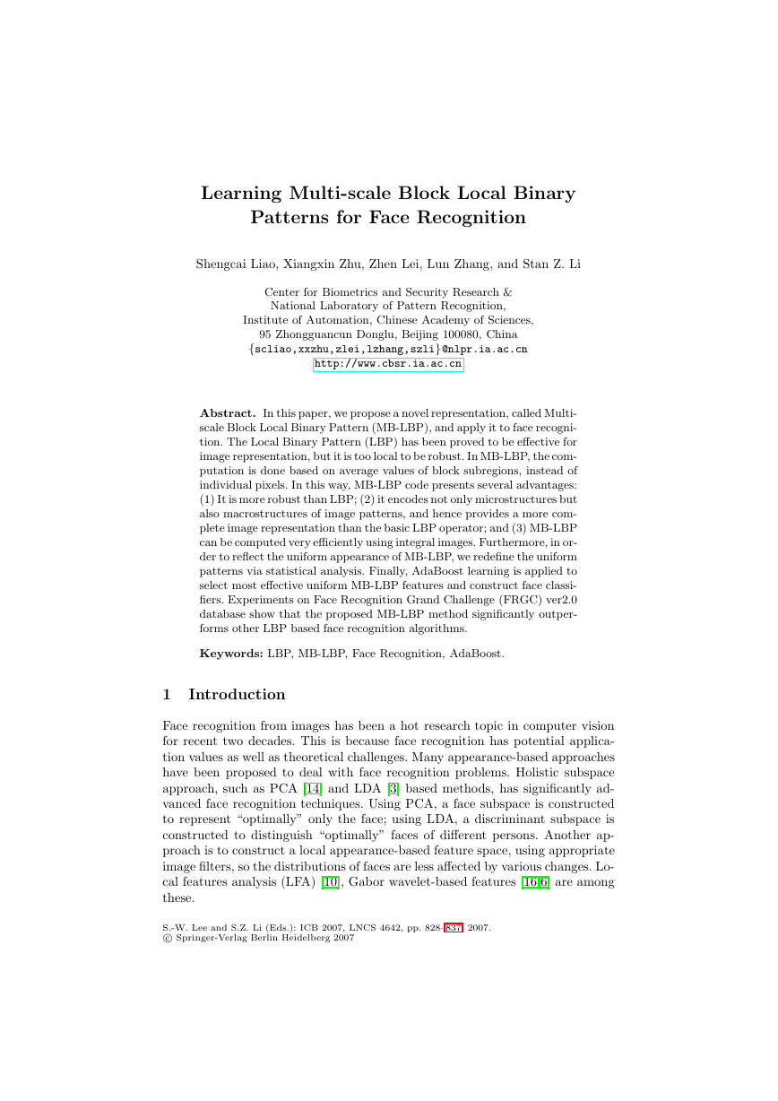
Fig. 1. (a) The basic LBP operator. (b) The 9×9 MB-LBP operator. In each sub-region,
average sum of image intensity is computed. These average sums are then thresholded
by that of the center block. MB-LBP is then obtained.
a binary string or a decimal number. Then the histogram of the labels can be
used as a texture descriptor. An illustration of the basic LBP operator is shown
in Fig. 1(a). Multi-scale LBP [9] is an extension to the basic LBP, with respect
to neighborhoods of different sizes.
In MB-LBP, the comparison operator between single pixels in LBP is simply
replaced with comparison between average gray-values of sub-regions (cf. Fig.
1(b)). Each sub-region is a square block containing neighboring pixels (or just
one pixel particularly). The whole filter is composed of 9 blocks. We take the
size s of the filter as a parameter, and s × s denoting the scale of the MB-LBP
operator (particularly, 3 × 3 MB-LBP is in fact the original LBP). Note that
the scalar values of averages over blocks can be computed very efficiently [13]
from the summed-area table [4] or integral image [15]. For this reason, MB-LBP
feature extraction can also be very fast: it only incurs a little more cost than the
original 3 × 3 LBP operator.
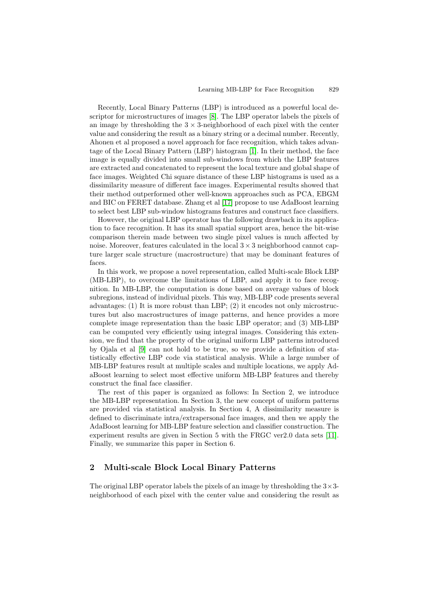
Fig. 2 gives examples of MB-LBP filtered face images by 3 × 3, 9 × 9 and
15 × 15 blocks. From this example we can see what influence parameter s would
make. For a small scale, local, micro patterns of a face structure is well rep-
resented, which may beneficial for discriminating local details of faces. On the
(a1)
(b1)
(c1)
(d1)
(a2)
(b2)
(c2)
(d2)
Fig. 2. MB-LBP filtered images of two different faces. (a) original images; (b) filtered
by 3 × 3 MB-LBP (c) filtered by 9 × 9 MB-LBP; (d) filtered by 15 × 15 MB-LBP.
�
Learning MB-LBP for Face Recognition
831
other hand, using average values over the regions, the large scale filters reduce
noise, and makes the representation more robust; and large scale information
provides complementary information to small scale details. But much discrimi-
native information is also dropped. Normally, filters of various scales should be
carefully selected and then fused to achieve better performance.
(a)
(b)
(c)
(d)
(e)
(f)
(g)
(h)
(i)
(j)
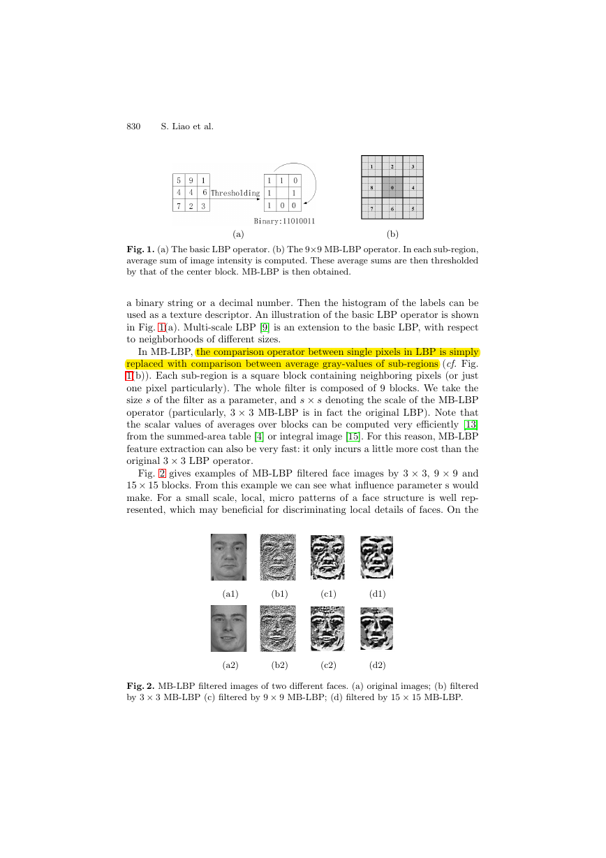
Fig. 3. Differential images. (a)(b) are the original intra-personal images, (c)(d)(e) are
the corresponding differential images generated by 3 × 3, 9 × 9 and 15 × 15 MB-
LBP operators. And (f)(g) are the original extra-personal images, (h)(i)(j) are the
corresponding differential images generated by 3 × 3, 9 × 9 and 15 × 15 MB-LBP
operators.
Fig. 3 demonstrates MB-LBP features for intra-personal and extra-personal
difference images (brighter pixels indicate greater difference). Using differential
images, We also have another way to demonstrate the discriminative power of
MB-LBP. We see that when scale of the MB-LBP filter become larger, thought
both intra-personal variance and extra-personal variance decrease, it is more
clear that with larger scale MB-LBP, intra-personal differences are smaller than
that of the extra-personal.
3 Statistically Effective MB-LBP (SEMB-LBP)
Using the “uniform” subset of LBP code improves the performance of LBP based
methods. A Local Binary Pattern is called uniform if it contains at most two
bitwise transitions from 0 to 1 or vice versa when the binary string is considered
circular [9]. It is observed that there are a limited number of transitions or
discontinuities in the circular presentation of the 3×3 texture patterns; according
to Ojala, this uniform patterns are fundamental properties of local image texture,
they provide a vast majority amount all patterns: 90% for (8,2) type LBP, 70%
for (16,2) type [9].
However, the original definition of uniform LBP patterns based on the tran-
sition of pixel values can not be used for MB-LBP with blocks containing more
�
832
S. Liao et al.
than a single pixel. The reason is obvious: the same properties of circular conti-
nuities in 3×3 patterns can not hold to be true when parameter s becomes larger.
Using average gray-values instead of single pixels, MB-LBP reflects the statisti-
cal properties of local sub-region relationship. The lager parameter s becomes,
the harder for the circular presentation to be continuous.
So we need to redefine uniform patterns. Since the term uniform refers to
the uniform appearance of the local binary pattern, we can define our uniform
MB-LBP via statistical analysis. Here, we present the concept of Statistically Ef-
fective MB-LBP (SEMB-LBP), based on the percentage in distributions, instead
of the number of 0-1 and 1-0 transitions as in the uniform LBP.
Denote fs(x, y) as an MB-LBP feature of scale s at location (x, y) computed
from original images. Then a histogram of the MB-LBP feature fs(·,·) over a
certain image I(x, y) can be defined as:
Hs(l) = 1[fs(x,y)=l],
= 0, . . . , L − 1
(1)
where 1(S) is the indicator of the set S, and is the label of the MB-LBP code.
Because all MB-LBP code are 8-bit binary string, so there are total L = 28 =
256 labels. Thus the histogram has 256 bins.
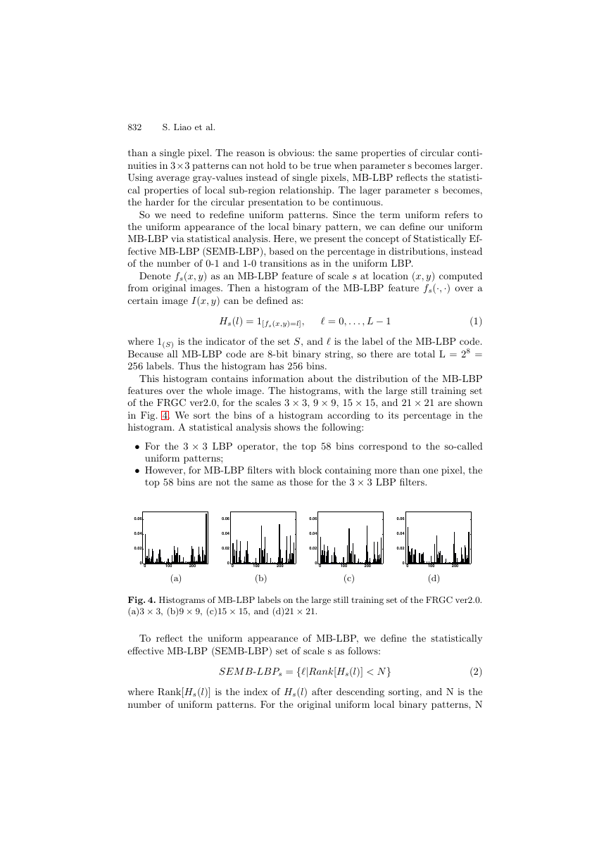
This histogram contains information about the distribution of the MB-LBP
features over the whole image. The histograms, with the large still training set
of the FRGC ver2.0, for the scales 3 × 3, 9 × 9, 15 × 15, and 21 × 21 are shown
in Fig. 4. We sort the bins of a histogram according to its percentage in the
histogram. A statistical analysis shows the following:
• For the 3 × 3 LBP operator, the top 58 bins correspond to the so-called
• However, for MB-LBP filters with block containing more than one pixel, the
uniform patterns;
top 58 bins are not the same as those for the 3 × 3 LBP filters.
0.06
0.04
0.02
0.06
0.04
0.02
0.06
0.04
0.02
0.06
0.04
0.02
0
0
100
200
0
0
100
200
0
0
100
200
0
0
100
200
(a)
(b)
(c)
(d)
Fig. 4. Histograms of MB-LBP labels on the large still training set of the FRGC ver2.0.
(a)3 × 3, (b)9 × 9, (c)15 × 15, and (d)21 × 21.
To reflect the uniform appearance of MB-LBP, we define the statistically
effective MB-LBP (SEMB-LBP) set of scale s as follows:
SEM B-LBPs = {|Rank[Hs(l)] < N}
(2)
where Rank[Hs(l)] is the index of Hs(l) after descending sorting, and N is the
number of uniform patterns. For the original uniform local binary patterns, N
�
Learning MB-LBP for Face Recognition
833
= 58. However, in our definition, N can be assigned arbitrarily from 1 to 256.
Large value of N will cause the feature dimensions very huge, while small one
loses feature variety. Consequently, we adopt N = 63 for a trade-off. Labeling all
remaining patterns with a single label, we use the following notation to represent
SEMB-LBP:
us(x, y) = { Indexs[fs(x, y)],
N,
if fs(x, y) ∈ SEM B-LBPs
otherwise
(3)
where Indexs[fs(x, y)] is the index of fs(x, y) in the set SEM B-LBPs (started
from 0).
4 AdaBoost Learning
The above SEMB-LBP provides an over-complete representation. The only ques-
tion remained is how to use them to construct a powerful classifier. Because those
excessive measures contain much redundant information, a further processing is
needed to remove the redundancy and build effective classifiers. In this paper
we use Gentle AdaBoost algorithm [5] to select the most effective SEMB-LBP
feature.
Boosting can be viewed as a stage-wise approximation to an additive logistic
regression model using Bernoulli log-likelihood as a criterion [5]. Developed by
Friedman et al, Gentle AdaBoost modifies the population version of the Real
AdaBoost procedure [12], using Newton stepping rather than exact optimiza-
tion at each step. Empirical evidence suggests that Gentle AdaBoost is a more
conservative algorithm that has similar performance to both the Real AdaBoost
and LogitBoost algorithms, and often outperforms them both, especially when
stability is an issue.
Face recognition is a multi-class problem whereas the above AdaBoost learning
is for two classes. To dispense the need for a training process for faces of a
newly added person, we use a large training set describing intra-personal or
extra-personal variations [7], and train a “universal” two-class classifier. An ideal
intra-personal difference should be an image with all pixel values being zero,
whereas an extra-personal difference image should generally have much larger
pixel values. However, instead of deriving the intra-personal or extra-personal
variations using difference images as in [7], the training examples to our learning
algorithm is the set of differences between each pair of local histograms at the
corresponding locations. The positive examples are derived from pairs of intra-
personal differences and the negative from pairs of extra-personal differences.
In this work, a weak classifier is learned based on a dissimilarity between two
corresponding histogram bins. Once the SEMB-LBP set are defined for each
scale, histogram of these patterns are computed for calculating the dissimilar-
ity: First, a sequence of m subwindows R0, R1, . . . , Rm−1 of varying sizes and
locations are obtained from an image; Second, a histogram is computed for each
SEMB-LBP code i over a subwindow Rj as
Hs,j(i) = 1[us(x,y)=i] · 1[(x,y)∈Rj],
i = 0, . . . , N, j = 0, . . . , m − 1
(4)
�
834
S. Liao et al.
The corresponding bin difference is defined as
s,j(i) − H 2
s,j(i)) = |H 1
s,j(i)|
D(H 1
s,j(i), H 2
i = 0, . . . , N
(5)
The best current weak classifier is the one for which the weighted intra-
personal bin differences (over the training set) are minimized while that of the
extra-personal are maximized.
With the two-class scheme, the face matching procedure will work in the
following way: It takes a probe face image and a gallery face image as the input,
and computes a difference-based feature vector from the two images, and then
it calculates a similarity score for the feature vector using the learned AdaBoost
classifier. Finally, A decision is made based on the score, to classify the feature
vector into the positive class (coming from the same person) or the negative
class (different persons).
5 Experiments
The proposed method is tested on the Face Recognition Grand Challenge (FRGC)
ver2.0 database [11]. The Face Recognition Grand Challenge is a large face recog-
nition evaluation data set, which contains over 50,000 images of 3D scans and
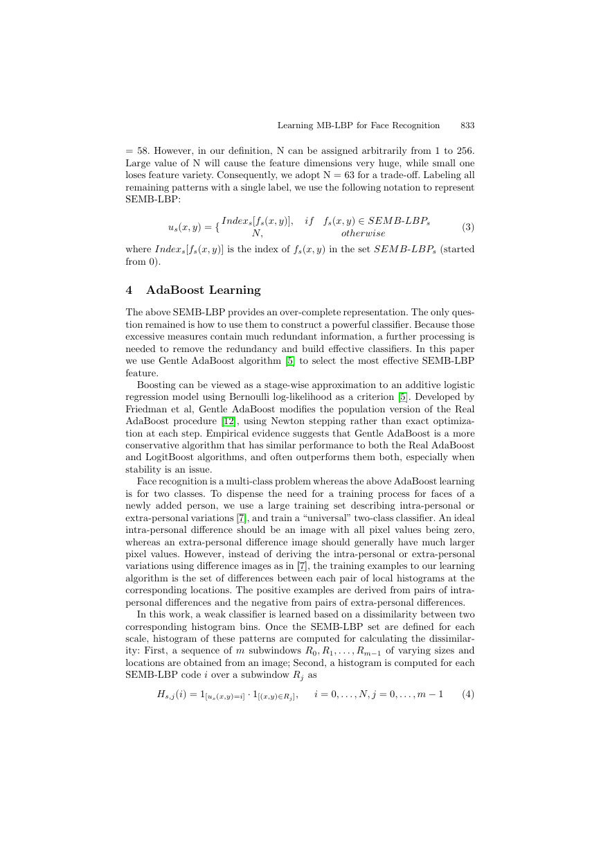
high resolution still images. Fig. 5 shows a set of images in FRGC for one sub-
ject section. The FRGC ver2.0 contains a large still training set for training still
face recognition algorithms. It consists of 12,776 images from 222 subjects. A large
validation set is also provided for FRGC experiments, which contains 466 subjects
from 4,007 subject sessions.
Fig. 5. FRGC images from one subject session. (a) Four controlled still images, (b)
two uncontrolled stills, and (c) 3D shape channel and texture channel pasted on the
corresponding shape channel.
The proposed method is evaluated on two 2D experiments of FRGC: Experi-
ment 1 and Experiment 2. Experiment 1 is designed to measure face recognition
performance on frontal facial images taken under controlled illumination. In this
experiment, only one single controlled still image is contained in one biometric
sample of the target or query sets. Experiment 2 measures the effect of multiple
�
Learning MB-LBP for Face Recognition
835
still images on performance. In Experiment 2, each biometric sample contains
four controlled images of a person taken in a subject session. There are 16 match-
ing scores between one target and one query sample. These scores are averaged
to give the final result.
There are total 16028 still images both in target and query sets of experiment
1 and 2. In the testing phase, it will generate a large similarity matrix of 16028
by 16028. Furthermore, three masks are defined over this similarity matrix, thus
three performance results will obtained, corresponding to Mask I, II, and III.
In mask I all samples are within semesters, in mask II they are within a year,
while in mask III the samples are between semesters, i.e., they are of increasing
difficulty.
In our experiments, All images are cropped to 144 pixels high by 112 pixels
wide, according to the provided eyes positions. A boosting classifier is trained
on the large still training set. The final strong classifier contains 2346 weak
classifiers, e.g. 2346 bins of various sub-region SEMB-LBP histograms, while
achieving zero error rate on the training set. The corresponding MB-LBP filter
size of the first 5 learned weak classifiers are s = 21, 33, 27, 3, 9. We find that a
middle level of scale s has a better discriminative power.
To compare the performances of LBP based methods, we also evaluate Ahonen
et al’s LBP method [1] and Zhang et al’s Boosting LBP algorithm [17]. We
use LBP u2
8,2 operator as Ahonen’s, and test it directly on FRGC experiment 1
and 2 since their method needs no training. For Zhang’s approach, we train an
AdaBoost classifier on the large still training set in the same way of our MB-
LBP. The final strong classifier of Zhang’s contains 3072 weak classifiers, yet it
can not achieve zero error rate on the training set.
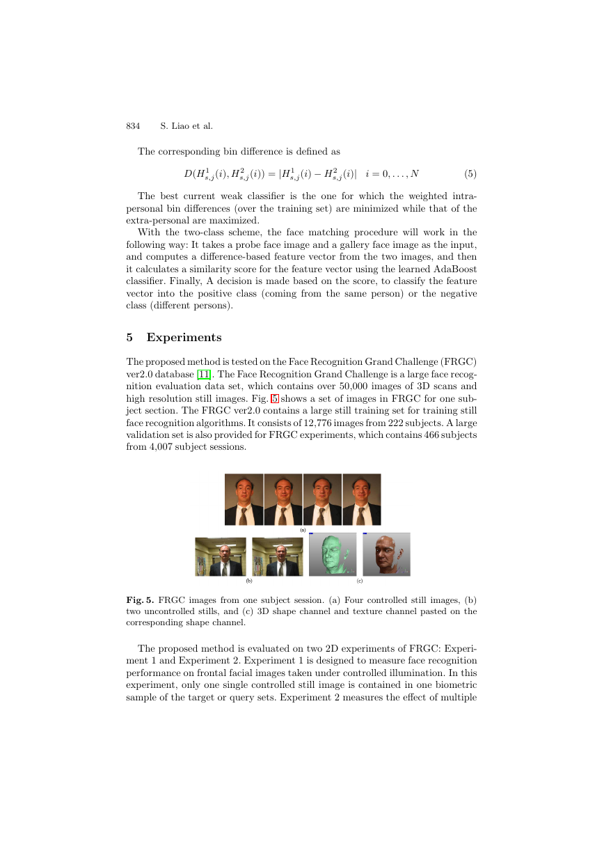
The comparison results are given in Fig. 6, and Fig. 7 describes the veri-
fication performances on a receiver operator characteristic(ROC) curve (mask
III). From the results we can see that MB-LBP outperforms the other two al-
gorithms on all experiments. The comparison proves that MB-LBP is a more
robust representation than the basic LBP. Meanwhile, because MB-LBP pro-
vides a more complete image representation that encodes both microstructure
and macrostructure, it can achieve zero error rate on the large still training set,
while generate well on the validation face images. Furthermore, we can also find
that MB-LBP performs well on Mask III, which means that it is robust with
time elapse.
Experiment 1
Experiment 2
MB-LBP
Zhang’s LBP 84.17
Ahonen’s LBP 82.72
Mask I Mask II Mask III Mask I Mask II Mask III
98.07 97.04
80.35
78.65
96.05 99.78 99.58
96.73
76.67
74.78
90.54
99.45
95.84
87.46
97.67
93.62
Fig. 6. Verification performance (FAR=0.1%) on FRGC Experiment 1 and 2
�


 2023年江西萍乡中考道德与法治真题及答案.doc
 2012年重庆南川中考生物真题及答案.doc
 2013年江西师范大学地理学综合及文艺理论基础考研真题.doc
 2020年四川甘孜小升初语文真题及答案I卷.doc
 2020年注册岩土工程师专业基础考试真题及答案.doc
 2023-2024学年福建省厦门市九年级上学期数学月考试题及答案.doc
 2021-2022学年辽宁省沈阳市大东区九年级上学期语文期末试题及答案.doc
 2022-2023学年北京东城区初三第一学期物理期末试卷及答案.doc
 2018上半年江西教师资格初中地理学科知识与教学能力真题及答案.doc
 2012年河北国家公务员申论考试真题及答案-省级.doc
 2020-2021学年江苏省扬州市江都区邵樊片九年级上学期数学第一次质量检测试题及答案.doc
 2022下半年黑龙江教师资格证中学综合素质真题及答案.doc