Nonlinear Dyn (2009) 55: 385–393
DOI 10.1007/s11071-008-9371-1
O R I G I N A L PA P E R
Neural networks based self-learning PID control
of electronic throttle
Xiaofang Yuan · Yaonan Wang
Received: 13 April 2008 / Accepted: 9 May 2008 / Published online: 3 June 2008
© Springer Science+Business Media B.V. 2008
Abstract An electronic throttle is a low-power DC
servo drive which positions the throttle plate. Its ap-
plication in modern automotive engines leads to im-
provements in vehicle drivability, fuel economy, and
emissions. In this paper, a neural networks based self-
learning proportional-integral-derivative (PID) con-
troller is presented for electronic throttle. In the pro-
posed self-learning PID controller, the controller pa-
rameters, KP , KI , and KD are treated as neural net-
works weights and they are adjusted using a neural
networks algorithm. The self-learning algorithm is op-
erated iteratively and is developed using the Lyapunov
method. Hence, the convergence of the learning algo-
rithm is guaranteed. The neural networks based self-
learning PID controller for electronic throttle is veri-
fied by computer simulations.
Keywords Nonlinear systems · Nonlinear control ·
Electronic throttle · PID control · Neural networks ·
Self-learning
1 Introduction
Today’s automobile effectively encompasses the spirit
of mechatronic systems with its abundant applica-
X. Yuan () · Y. Wang
College of Electrical and Information Engineering, Hunan
University, Changsha 410082, China
e-mail: yuanxiaofang126@126.com
tion of electronics, sensors, actuators, and micro-
processor-based control systems to provide improved
performance,
fuel economy, emission levels, and
safety. Electronic throttle is a DC motor driven valve
that regulates air inflow into the engine’s combus-
tion system [1]. Electronic throttle can successfully
replace its mechanical counterpart if a control loop
satisfies prescribed requirements: a fast transient re-
sponse without overshoot, positioning within the mea-
surement resolution, and the control action that does
not wear out the components. Vehicles equipped with
electronic throttle control (ETC) systems are gain-
ing popularity in the automotive industry for several
reasons including improved fuel economy, vehicle
drivability, and emissions. As adaptive-cruise-control
and direct-fuel-injection systems become popular, the
market of ETC has become larger [2]. The ETC system
positions the throttle valve according to the reference
opening angle provided by the engine control unit. To-
day’s engine control unit use lookup tables with sev-
eral thousand entries to find the fuel and air combina-
tion which maximizes fuel efficiency and minimizes
emissions while respecting drivers intentions. Hence,
accurate and fast following of the reference opening
angle by the electronic throttle has direct economical
and ecological impacts.
The synthesis of a satisfactory ETC system is diffi-
cult since the plant is burdened with strong nonlinear
effects of friction and limp-home nonlinearity. More-
over, the control strategy should be simple enough
�
386
to be implemented on a typical low-cost automotive
micro-controller system, while it has to be robust for a
range of plant parameters variations. Additionally, the
control strategy should respect physical limitations of
the throttle control input and safety constraints on the
plant variables prescribed by the manufacturer.
Considering everything mentioned before, it is not
a surprise that this challenging control problem has at-
tracted significant attention of the research community
in the last decade [3–9]. There are several ETC con-
trol strategies that differ in the underlying philosophy,
complexity, and the number of sensor signals needed
to determine the desired throttle opening. Several of
the existing control strategies use a linear model of
the plant and derive a proportional-integral-derivative
(PID) controller with feedback compensator [3]. Vari-
able structure control with sliding mode is an effec-
tive method for the control of nonlinear plant with pa-
rameter uncertainty, and it has also been applied in
the ETC system in [4, 5], and [6]. In [4], a discrete-
time sliding mode controller and observer are designed
to realize ETC system by replacing signum functions
with continuous approximations. A sliding model con-
troller coupled with a genetic algorithm (GA) based
variable structure system observer fulfills the demand
for high robustness in nonlinear opening of the throt-
tle in [5]. In [6], a neural networks based sliding mode
controller is described since neural networks has good
learning ability and nonlinear approximation capabil-
ity. In [7], variable structure control technique based
robust control is presented. A time-optimal model pre-
dictive control is proposed in [8] based on the discrete-
time piecewise affine model of the throttle. In [9], re-
current neuro-controller is trained for real time appli-
cation in the electronic throttle and hybrid electric ve-
hicle control.
It is well known that proportional-integral-deriva-
tive (PID) controllers have dominated industrial con-
trol applications for a half of century, although there
has been considerable research interest in the imple-
mentation of advanced controllers. This is due to the
fact that the PID control has a simple structure that
is easily understood by field engineers and is robust
against disturbance and system uncertainty. As most
of the industrial plants demonstrate nonlinearity in the
system dynamics in a wide operating range, different
PID control strategies have been investigated in the
past years.
In this paper, a neural networks based self-learning
PID controller is proposed for the ETC system. The
X. Yuan, Y. Wang
proposed self-learning PID controller is also accept-
able in engineering practice as it can meet the follow-
ing requirements: (1) Fulfill the demand of total non-
linear characteristic in throttle, i.e., stick-slip friction,
nonlinear spring, and gear backlash. (2) Simplicity of
the control strategy is required, so that it can be imple-
mented on a low-cost automotive micro-controller sys-
tem. (3) Robustness of the control system with respect
to variations of plant parameters is required, which can
be caused by production deviations, variations of ex-
ternal conditions. (4) Settling time of the position con-
trol system step response should be less than 0.15 sec-
onds for any operating point and for any reference step
change.
This paper is organized as follows. In Sect. 2, the
nonlinear dynamics of electronic throttle is derived.
In Sect. 3, a self-learning PID controller is presented
and it is implemented using neural networks approach.
At last, several simulations illustrate the performance
of the proposed self-learning PID controller for elec-
tronic throttle.
2 Model of electronic throttle
The electronic throttle consists of a DC drive (powered
by the chopper), a gearbox, a valve plate, a dual return
spring, and a position sensor. All throttle components
are assembled in a compact electronic throttle body as
in Fig. 1, which is mounted on the engine air tube. The
control signal is fed to the bipolar chopper, which sup-
plies the DC drive with the appropriate armature volt-
age. The armature current created induces the motor
torque that is transmitted through the gearbox to the
throttle plate. The valve plate movement stops when
the motor torque is counterbalanced by the torque of
the dual return spring, the gearbox friction torque, and
the load torque induced by the air inflow.
The complete electronic throttle plant can be given
by [10]:
˙θ = ω
˙w = − Ks
+ KT
J
J
VBat
Ra + RBat
J
θ − Cs
− K
d
J
ω − Kf
J
sgn(ω)
u
(1)
where θ is the throttle angle; ω is the throttle angular
velocity; J is lumped inertia of throttle plate, reduc-
tion gears and motor rotor; Ks is spring constant; Cs is
torque constant (spring torque at θ = 0); K
d is equiv-
�
Neural networks based self-learning PID control of electronic throttle
387
Fig. 1 The structure of an
electronic throttle
alent viscous friction constant, while Kf is Coulomb
friction constant; KT is motor torque constant; VBat is
no-load voltage; sgn(·) is the signum function; Ra is
armature resistance; RBat is internal resistance of the
source; u is the control signal. In the electronic throt-
tle control system, the throttle angle θ is the control
objective, and u is the control input then:
θ − Cs
− K
d
J
˙θ − Kf
J
sgn(˙θ )
¨θ = − Ks
+ KT
J
J
VBat
Ra + RBat
u
J
we also can present the plant as:
¨θ = f (θ, ˙θ ) + bu + d(t )
y = θ
(2)
(3)
where f is a unknown function, b is a unknown pa-
rameter, but it is assumed to be a constant, d(t ) is
the unknown external disturbance, u ∈ R and y ∈ R
are the input and output of the plant, respectively,
θ = (θ, ˙θ )T ∈ Rn is the state vector of the plant, which
is assumed to be measurable. And it is assumed that
d(t ) have upper bound D, that is, |d(t )| ≤ D.
3 Self-learning PID controller design
3.1 PID control
In control engineering, PID control technique has been
considered as a matured technique in comparing with
other control techniques. In a typical discrete-time PID
controller, its control law can be expressed in the fol-
lowing forms [11, 12]:
u(k) = KP (k)e(k) + KI (k)
ei (k) + KD(k)e(k)
(4)
i
∗
where KP (k), KI (k) and KD(k) are proportional, in-
tegral, and derivative gains, respectively; u(k) is an
overall control force at time k which is a summation
of three components; e(k) is the tracking error defined
as: e(k) = y
(k)− y(k), and e(k) = e(k)− e(k − 1);
∗
(k) is the desired plant output, y(k) is the actual
y
plant output at time k. We also can present the PID
control in the increment forming as:
u(k) = u(k − 1) + u(k)
u(k) = 3
Ki (k) · ei (k)
i=1
(k) − y(k), e2(k) = e1(k) − e1(k −
where e1(k) = y
1), e3(k) = e1(k) − 2e1(k − 1) + e1(k − 2); Ki
(i = 1, 2, 3) are the three parameters for PID control,
if we can select the optimal values of Ki (i = 1, 2, 3),
the PID controller will have good performance. How-
ever, these parameters are not easy to select since the
practical plant is generally nonlinear. In this paper, we
will propose an intelligent PID controller as the para-
meters of PID controller used here can adjust its pa-
rameters in an intelligent way, which is implemented
using neural networks.
(5)
∗
3.2 Structure of self-learning PID control
The structure of the proposed self-learning PID con-
troller is illustrated in Fig. 2. There are two neural net-
works; one is a Gaussian potential function networks
(GPFN1), which can identify the nonlinear plant, the
other is another Gaussian potential function networks
(GPFN2), which acts as a PID controller.
GPFN networks may be seen as a three-layer feed-
forward networks, the input layer acts as transmit-
ting input value to the next layer, the second layer is
a hidden-layer, center parameter is included in each
node, the third layer is output layer. Usually, nonlinear
�
388
X. Yuan, Y. Wang
Fig. 2 The structure of self-learning PID controller
plant could be described by nonlinear mapping shown
as follows:
y(k − 1), . . . , y(k − n), u(k), . . . , u(k − d)
y(k) = f
(6)
where n and d are orders of the plant output and con-
trol input. The GPFN1 is used for the construction of
plant model and input layer of GPFN1 is defined as:
y(k−1), . . . , y(k−n), u(k), . . . , u(k−d)
(7)
Xm(k) =
T
then the hidden layer of GPFN1 is
−Xm(k) − am
j (k) = exp
hm
j (k))2
j = 1, 2, . . . , M
2(bm
j (k)2
,
(8)
and the output layer of GPFN1 is obtained as
(9)
W m
j (k)
j (k) · hm
ˆy(k) = M
j=1
j (k) (j = 1, 2, . . . , M) are the networks con-
where W m
necting weights, am
j (k) is the center of the Gaussian
potential function, and bm
j (k) is the width of the
Gaussian potential function, at time k. ˆy(k) in (9) is
the approximation of y(k) in (6), and it constructs the
plant model.
GPFN2 acts as the self-learning PID controller, and
the output of GPFN2 is
u(k) = u(k − 1) + 3
i=1
Ki (k) · Φi (k)
and the hidden layer of GPFN2 is
−X(k) − ai (k)2
Φi (k) = exp
i = 1, 2, 3
i (k)
2b2
,
(10)
(11)
T
and the input layer of GPFN2 is
X1(k), X2(k), X3(k)
X(k) =
(12)
where Ki (k) (i = 1, 2, 3) is the networks connecting
weights, which is corresponding to PID controller pa-
rameters (proportional gains, integral gains, and deriv-
ative gains), X1(k) = e1(k), X2(k) = e2(k), X3(k) =
e3(k), ai (k) is the center of the Gaussian potential
function, and bi (k) is the width of the Gaussian po-
tential function at time k.
3.3 Learning algorithm
In this section, we will present the learning algorithm
for these two GPFN networks. For GPFN1, a cost
function may be defined as
2 = 1
Jm = 1
2
2
y(k) − ˆy(k)
e2
m(k)
(13)
�
Neural networks based self-learning PID control of electronic throttle
389
A gradient descent approach is employed to train
GPFN1 in order to minimize const function Jm.
The gradients of error in (13) with respect to vector
j (k), am
W m
The gradients of error in (20) with respect to vector
Ki (k), ai (k), and bi (k) are given by
· ∂y(k)
(k) − y(k)
= −
∂Jc
∗
y
∂u(k)
∂Ki (k)
= −e(k) · Φi (k) · ∂y(k)
= −
(k) − y(k)
∂u(k)
· ∂y(k)
∗
y
∂u(k)
(14)
∂Jc
∂ai (k)
· ∂u(k)
∂Ki (k)
· ∂u(k)
∂Φi (k)
∂Jm
∂W m
j (k)
∂Jm
j (k)
∂am
∂Jm
j (k)
∂bm
i (k) are given by:
· ∂ ˆy(k)
∂W m
j (k)
y(k) − ˆy(k)
i (k), and bm
= −
= em(k) · hm
j (k)
= −
y(k) − ˆy(k)
= −em(k) · W m
× Xm(k) − am
j (k))2
= −
y(k) − ˆy(k)
= −em(k) · W m
× Xm(k) − am
j (k))3
(bm
(bm
· ∂ ˆy(k)
∂hm
j (k)
j (k) · hm
j (k)
j (k)
· ∂ ˆy(k)
∂hm
j (k)
j (k) · hm
j (k)2
j (k)
The corresponding learning algorithm of GPFN1 are
given by the following expressions:
W m
j (k − 1) − W m
− ∂Jm
j (k − 1) + η(k) ·
j (k) = W m
∂W m
j (k)
j (k − 2)
+ α
W m
− ∂Jm
j (k) = am
j (k − 1) + η(k) ·
∂am
j (k)
j (k − 2)
j (k − 1) − am
+ α
j (k) = bm
j (k − 1) + η(k) ·
− ∂Jm
∂bm
j (k)
j (k − 2)
j (k − 1) − bm
+ α
am
bm
am
bm
(17)
(18)
(19)
where η(k) is the learning rate, 0 < η(k) < 1; α is pos-
itive factor.
Define a cost function for the online learning of
GPFN2 as:
∗
y
Jc = 1
2
(k) − y(k)
2 = 1
2
e2(k)
× ∂Φi (k)
∂ai (k)
= −e(k) · Ki (k) · Φi (k)
× (X(k) − ai (k))T
= −
b2
i (k)
(k) − y(k)
∗
y
· ∂y(k)
∂u(k)
· ∂y(k)
∂u(k)
· ∂hm
∂am
j (k)
j (k)
· ∂hm
∂bm
j (k)
j (k)
(15)
(16)
∂Jc
∂bi (k)
× ∂u(k)
∂Φi (k)
· ∂Φi (k)
∂bi (k)
= −e(k) · Ki · Φi (k)
× X(k) − ai (k)2
b3
i (k)
· ∂y(k)
∂u(k)
(23)
In these equations, ∂y(k)
∂u(k) denotes the sensitivity of
the plant with respect to its input, which is identified
using GPFN1 since after learning there is ˆy(k) ≈ y(k),
∂y(k)
∂u(k)
As
∂ ˆy(k)
∂u(k)
≈ ∂ ˆy(k)
∂u(k) .
= ∂ ˆy(k)
∂hm
j (k)
· ∂hm
j (k)
∂u(k)
j (k) · hm
W m
j (k) · hm
W m
= − M
j=1
= − M
j=1
j (k)
j (k) · X(k) − am
j (k)
j (k) · u(k) − am
j (k))2
(bm
(bm
j (k))2
therefore, the learning algorithms for GPFN2 are:
Ki (k) = Ki (k − 1) + η(k) ·
+ α
− ∂Jc
∂Ki (k)
Ki (k − 1) − Ki (k − 2)
− ∂Jc
∂ai (k)
ai (k − 1) − ai (k − 2)
ai (k) = ai (k − 1) + η(k) ·
(20)
+ α
(21)
(22)
(24)
(25)
(26)
�
390
bi (k) = bi (k − 1) + η(k) ·
− ∂Jc
∂bi (k)
bi (k − 1) − bi (k − 2)
+ α
(27)
where η(k) is the learning rate, 0 < η(k) < 1; α is pos-
itive factor.
For a proper understanding and applying the ap-
the more detailed procedures of the self-
proach,
learning PID control design are given below.
Step 1. Initial parameters: weights W m(0), K(0), pa-
i (0), bm
i (0), ai (0), bi (0), η = 0.35,
Step 2. Using (9) to compute the output of GPFN1
rameters am
α = 0.2.
ˆy(k).
Step 3. Using (14)–(16) and (17)–(19) to train the
weights and parameters of GPFN1.
Step 4. Compute ∂y(k)
Step 5. Sample y
∂u(k) using (24).
∗
(k), y(k), compute the control sig-
nal u(k) by (10).
Step 6. Update PID parameters (GPFN2) using (21)–
(23) and (25)–(27), go to Step 2.
3.4 Stability and convergence
The learning algorithms of GPFN2 in (25)–(27) can
be denoted as follows, that is, the weights can now be
adjusted following a gradient method as:
Wi (k) = Wi (k + 1) − Wi (k)
= −η(k) ·
∂Jc
∂Wi (k)
(28)
∂W (k) , g[ei (k)] = ∂Jc
where Wi (k) is the weights and parameters of GPFN2,
is, Wi (k) = [Ki (k), ai (k), bi (k)], η(k) is the
that
learning rate, 0 < η(k) < 1.
Let z(k) = ∂y(k)
learning rate as η(k) =
Therefore,
Wi (k + 1) = Wi (k) − η(k) ·
∂y(k) , and select the
1+z(k)2 , γ > 0 is a constant.
∂Jc
γ
∂Wi (k)
= Wi (k) − η(k) · ∂Jc
= Wi (k) − γ · g[e(k)]
1 + zT (k) · z(k)
∂y(k)
· ∂y(k)
∂W (k)
· z(k)
(29)
Assumption (1) 2 > γ > 0; (2) W (k) is very close to
optimal weights W
; (3) g(0) = 0.
∗
X. Yuan, Y. Wang
Theory Under Assumptions
is
limk→∞ g2[ei (k)]
= 0. And if z(k) is bounded,
1+zT (k)·z(k)
limk→∞ g[e(k)] = 0, limk→∞ e(k) → 0, and the learn-
ing algorithm is converged.
(1)–(3),
there
Proof Suppose weights W (k) are very close to opti-
mal weights W
be expressed by:
∗ = [ ¯W1, ¯W2, ¯W3], then (10) can
, W
∗
u(k) = 3
¯Wi (k) · Φi (k)
i=1
˜W (k) = W
∗ − W (k)
Define a Lyapunov function as
V (k) = ˜W (k)
2 ≥ 0
(30)
(31)
(32)
then
V (k + 1) = ˜W (k + 1)
2 = ˜W T (k + 1) ˜W (k + 1)
T
=
˜W (k) − γ · g[e(k)] · z(k)
1 + zT (k) · z(k)
˜W (k) − γ · g[e(k)] · z(k)
×
1 + zT (k) · z(k)
2 − 2γ ˜W T (k) · g[e(k)] · z(k)
= ˜W (k)
+ γ 2 · g2[e(k)] · zT (k) · z(k)
≤ V (k) − 2γ ˜W T (k) · g[e(k)] · z(k)
+ γ 2 · g2[e(k)]
1 + zT (k) · z(k)
[1 + zT (k) · z(k)]2
1 + zT (k) · z(k)
1 + zT (k) · z(k)
(33)
From Assumption (2) and (33), we can know
˜W T (k) · z(k) is the first order approximation of
that
g[e(k)], that is,
˜W T (k) · z(k) = ¯W − W (k)
+ o(1)
ei (k)
= g
T · ∂y(k)
∂W (k)
(34)
thus, the change of the Lyapunov function is obtained
by
�
Neural networks based self-learning PID control of electronic throttle
V (k) = V (k + 1) − V (k)
1 + zT (k) · z(k)
≥ − 2γ ˜W T (k) · g[e(k)] · z(k)
+ γ 2 · g2[e(k)]
1 + zT (k) · z(k)
≥ − γ (2 − γ ) · g2[e(k)]
1 + zT (k) · z(k)
(35)
When Assumption (1) is satisfied, 2 > γ > 0,
V (k) is negative definite. This also means that the
convergence is guaranteed, then limk→∞ g2[ei (k)]
=
1+zT (k)·z(k)
0, limk→∞ g[e(k)] = 0, limk→∞ e(k) → 0.
4 Simulation
d
J
= 2.01E02 rad/s2, K
= 3.30E01 s
= 2.50E01 rad/A · s2,
This section shows the application of the self-learning
PID controller on the electronic throttle. In this pa-
−2,
per, plant parameters values are: Ks
J
=
Cs
=
J
6.29E01 rad/s2, KT
J
3.0E01 A. Here, three kinds of controllers are com-
pared together. They are: PID controller with feed-
back compensator (PIDFC) in [3], recurrent neuro-
controller (RNC) in [9], and the proposed self-learning
PID controller (SLPID).
= 1.35E01 s
−1, Kf
Ra+RBat
J
VBat
Several set-points tracking are performed in this
simulation with different operating points and differ-
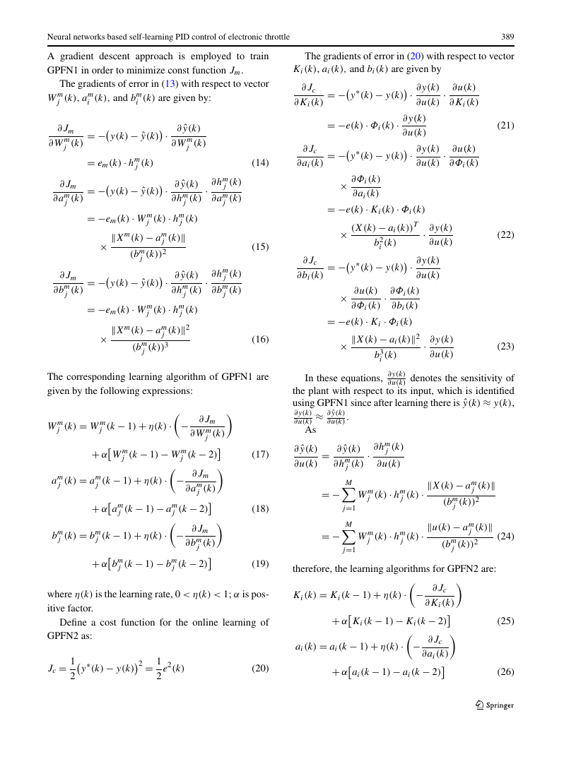
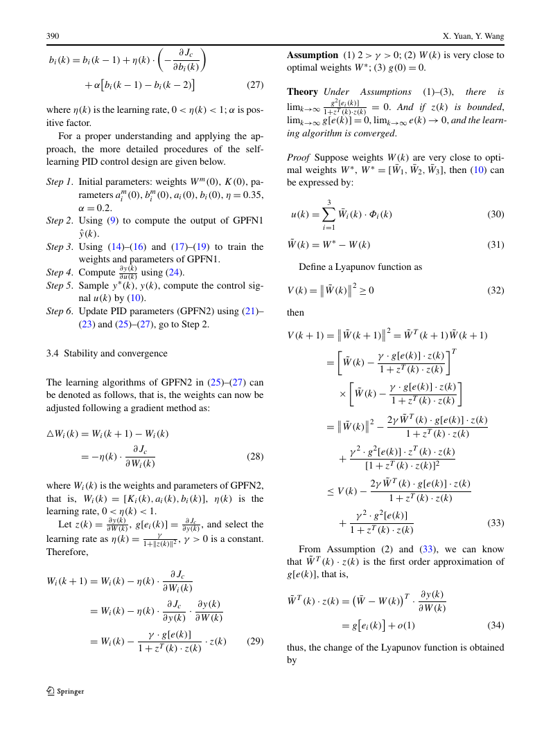
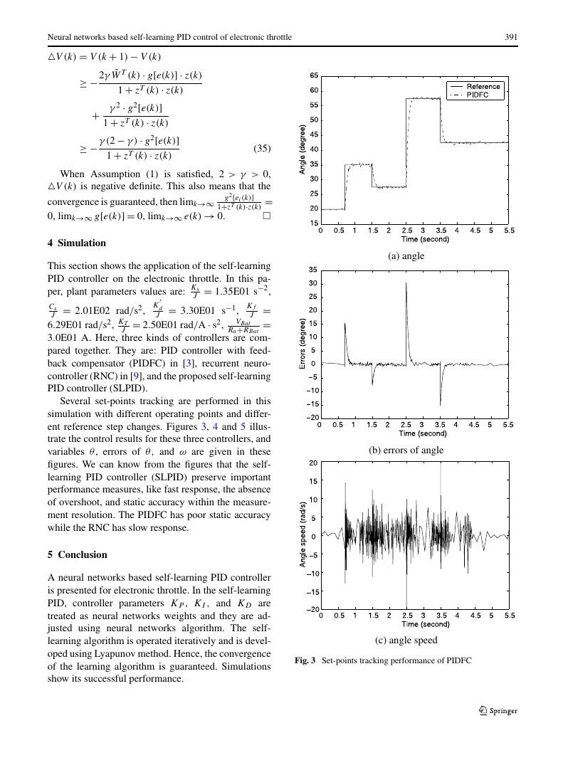
ent reference step changes. Figures 3, 4 and 5 illus-
trate the control results for these three controllers, and
variables θ, errors of θ, and ω are given in these
figures. We can know from the figures that the self-
learning PID controller (SLPID) preserve important
performance measures, like fast response, the absence
of overshoot, and static accuracy within the measure-
ment resolution. The PIDFC has poor static accuracy
while the RNC has slow response.
5 Conclusion
A neural networks based self-learning PID controller
is presented for electronic throttle. In the self-learning
PID, controller parameters KP , KI , and KD are
treated as neural networks weights and they are ad-
justed using neural networks algorithm. The self-
learning algorithm is operated iteratively and is devel-
oped using Lyapunov method. Hence, the convergence
of the learning algorithm is guaranteed. Simulations
show its successful performance.
391
(a) angle
(b) errors of angle
(c) angle speed
Fig. 3 Set-points tracking performance of PIDFC
�
392
X. Yuan, Y. Wang
(a) angle
(a) angle
(b) errors of angle
(b) errors of angle
(c) angle speed
(c) angle speed
Fig. 4 Set-points tracking performance of RNC
Fig. 5 Set-points tracking performance of SLPID
�


 2023年江西萍乡中考道德与法治真题及答案.doc
 2012年重庆南川中考生物真题及答案.doc
 2013年江西师范大学地理学综合及文艺理论基础考研真题.doc
 2020年四川甘孜小升初语文真题及答案I卷.doc
 2020年注册岩土工程师专业基础考试真题及答案.doc
 2023-2024学年福建省厦门市九年级上学期数学月考试题及答案.doc
 2021-2022学年辽宁省沈阳市大东区九年级上学期语文期末试题及答案.doc
 2022-2023学年北京东城区初三第一学期物理期末试卷及答案.doc
 2018上半年江西教师资格初中地理学科知识与教学能力真题及答案.doc
 2012年河北国家公务员申论考试真题及答案-省级.doc
 2020-2021学年江苏省扬州市江都区邵樊片九年级上学期数学第一次质量检测试题及答案.doc
 2022下半年黑龙江教师资格证中学综合素质真题及答案.doc