GLMix: Generalized Linear Mixed Models For Large-Scale
Response Prediction
Xianxing Zhang, Yitong Zhou, Yiming Ma, Bee-Chung Chen, Liang Zhang, Deepak Agarwal
{xazhang, yizhou, yma, bchen, lizhang, dagarwal}@linkedin.com
LinkedIn
Mountain View, CA, USA
ABSTRACT
Generalized linear model (GLM) is a widely used class of
models for statistical inference and response prediction prob-
lems. For instance, in order to recommend relevant content
to a user or optimize for revenue, many web companies use
logistic regression models to predict the probability of the
user’s clicking on an item (e.g., ad, news article, job).
In
scenarios where the data is abundant, having a more fine-
grained model at the user or item level would potentially
lead to more accurate prediction, as the user’s personal pref-
erences on items and the item’s specific attraction for users
can be better captured. One common approach is to in-
troduce ID-level regression coe�cients in addition to the
global regression coe�cients in a GLM setting, and such
models are called generalized linear mixed models (GLMix)
in the statistical literature. However, for big data sets with a
large number of ID-level coe�cients, fitting a GLMix model
can be computationally challenging. In this paper, we re-
port how we successfully overcame the scalability bottleneck
by applying parallelized block coordinate descent under the
Bulk Synchronous Parallel (BSP) paradigm. We deployed
the model in the LinkedIn job recommender system, and
generated 20% to 40% more job applications for job seekers
on LinkedIn.
1.
INTRODUCTION
Accurate prediction of users’ responses to items is one
of the core functions of many recommendation applications.
Examples include recommending movies, news articles, songs,
jobs, advertisements, and so forth. Given a set of features,
a common approach is to apply generalized linear models
(GLM). For example, when the response is numeric (e.g.,
rating of a user to a movie), a linear regression on the fea-
tures is commonly used to predict the response. For the
binary response scenario (e.g. whether to click or not when
a user sees a job recommendation), logistic regression is of-
ten used. Sometimes the response is a count (e.g., number
of times a user listens to a song), and Poisson regression be-
Permission to make digital or hard copies of all or part of this work for personal or
classroom use is granted without fee provided that copies are not made or distributed
for profit or commercial advantage and that copies bear this notice and the full cita-
tion on the first page. Copyrights for components of this work owned by others than
ACM must be honored. Abstracting with credit is permitted. To copy otherwise, or re-
publish, to post on servers or to redistribute to lists, requires prior specific permission
and/or a fee. Request permissions from permissions@acm.org.
KDD ’16 Aug 13–17, 2016, San Francisco, CA, USA
c� 2016 ACM. ISBN 978-1-4503-4232-2/16/08. . . $15.00
DOI: http://dx.doi.org/10.1145/2939672.2939684
comes a natural choice. All of the above models are special
cases of GLM.
The features available in recommender systems often in-
clude user features (e.g., age, gender, industry, job func-
tion) and item features (e.g., title and skills for jobs, title
and named entities for news articles). An approach that is
widely adopted in industry to model interactions between
users and items is to form the outer (cross) product of user
and item features, followed by feature selection to reduce the
dimensionality and mitigate the problem of overfitting. In
reality, we often observe a lot of heterogeneity in the amount
of data per user or item that cannot be su�ciently modeled
by user/item features alone, which provides an opportunity
to improve model accuracy by adding more granularity to
the model. Specifically, for a user who has interacted with
many items in the past, we should have su�cient data to fit
regression coe�cients that are specific to that user to cap-
ture his/her personal interests. Similarly, for an item that
has received many users’ responses, it is beneficial to model
its popularity and interactions with user features through
regression coe�cients that are specific to the item.
One common approach to capture such behavior of each
individual user and item is to use ID-level features, i.e., the
outer product of user IDs and item features, and the outer
product of item IDs and user features. Models with ID-level
features are usually referred to as generalized linear mixed
models (GLMix) in Statistics [15]. Although conceptually
simple, it can generate a very large number of regression
coe�cients to be learned. For example, for a data set of
10 million users, and each user with 1,000 non-zero coe�-
cients on item features, the total number of regression coef-
ficients can easily go beyond 1010. Therefore, fitting GLMix
models for big data is computationally challenging. Dimen-
sion reduction methods such as feature hashing [1] or princi-
pal component analysis can reduce the number of features.
However, they also reduce our ability to interpret the model
or explain the predictions in the original feature space (e.g.,
at the user’s ID level), making it di�cult to debug or inves-
tigate system issues or user complaints.
1.1 Our contributions
In this paper we develop a parallel block-wise coordinate
descent (PBCD) algorithm under the Bulk Synchronous Par-
allel (BSP) paradigm [21] for GLMix model, with a novel
model score movement scheme that allows both the coe�-
cients and the data to stay in local nodes. We show that
our algorithm successfully scales model fitting of GLMix for
very large data sets. We empirically demonstrate that this
conceptually simple class of models achieves high accuracy
�
bers to connect with all kinds of professional opportunities
for their career growth. One of the most important products
is the Jobs Homepage, which serves as a central place for
members with job seeking intention to come and find good
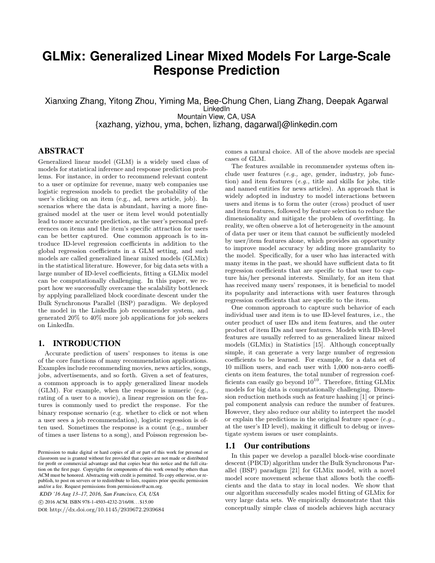
jobs to apply for. Figure 1 is a snapshot of the LinkedIn
Jobs Homepage. One of the main modules on the page is
“Jobs you may be interested in”, where relevant job thumb-
nails are recommended to members based on their public
profile data and past activity on the site.
If a member is
interested in a recommended job, she can click on it to go
to the job detail page, where the original job post is shown
with information such as the job title, description, respon-
sibilities, required skills and qualifications. The job detail
page also has an “apply” button which allows the member
to apply for the job with one click, either on LinkedIn or on
the website of the company posting the job. One of the key
success metrics for LinkedIn jobs business is the total num-
ber of job application clicks (i.e the number of clicks on the
“apply” button), which is the focus for the job recommenda-
tion problem in this paper. Another second-order metric is
called “job detail views”, which represents the total number
of clicks generated from the “Jobs you may be interested in”
module to the job details pages. We consider job applica-
tion clicks to be the key metric to optimize for, instead of
job detail views, because the job posters mostly care about
how many applications they receive, instead of how many
people view their job postings.
2.2 GLMix Model
Now we consider the GLMix model for the job recommen-
dation problem. To measure whether job j is a good match
for a member m and to select the best jobs according to this
measure, the key is to predict the probability that member
m would apply for job j given an impression on the “Jobs
you may be interested in” module. Let ymjt denote the bi-
nary response of whether member m would apply for job j
in context t, where the context usually includes the time and
location where the job is shown. We use qm to denote the
feature vector of member m, which includes the features ex-
tracted from the member’s public profile, e.g., the member’s
title, job function, education history, industry, etc. We use
sj to denote the feature vector of job j, which includes fea-
tures extracted from the job post, e.g. the job title, desired
skills and experiences, etc. Let xmjt represent the overall
feature vector for the (m, j, t) triple, which can include qm
and sj for feature-level main e↵ects, the outer product be-
tween qm and sj for interactions among member and job
features, and features of the context. We assume that xmjt
does not contain member IDs or item IDs as features, be-
cause IDs will be treated di↵erently from regular features.
The GLMix model for predicting the probability of mem-
ber m applying for job j using logistic regression is:
g(E[ymjt]) = x0mjtb + s0j↵m + q0m�j,
(1)
where g(E[ymjt]) = log E[ymjt]
1�E[ymjt] is the link function, b is
the global coe�cient vector (also called fixed e↵ect coe�-
cients in the statistical literature); and ↵m and �j are the
coe�cient vectors specific to member m and job j, respec-
tively. ↵m and �j are called random e↵ects coe�cients,
which capture member m’s personal preference on di↵erent
item features and item j’s attraction for di↵erent member
features.
Figure 1: A snapshot of the LinkedIn jobs homepage.
on two public data sets and the LinkedIn job recommenda-
tion data set. We also report our successful deployment of
GLMix in LinkedIn’s job recommendation production sys-
tem, which improved the total number of job applications
from active job seekers by 20% to 40%. To our knowledge,
this is the first paper that discusses the practical lessons
learned to scale GLMix in real web recommender system
applications.
We also extend GLMix by adding a matrix factorization
component in order to further leverage recent advancements
in scaling up matrix factorization in the distributed environ-
ment [24], and see some slight improvement on LinkedIn job
recommendation data. Since the parallelization of matrix
factorization is well studied, in this paper we mainly focus
on the scalability and parallelization of fitting GLMix.
We provide an implementation of the GLMix model with
Apache Spark1, and the code base is open sourced as part
of the Photon-ML library2.
1.2 Organization
The paper is organized as follows. We start by introducing
the LinkedIn job recommendation problem as our motivat-
ing example and describing the formulation of the GLMix
model in such a context in Section 2. The fitting algorithm
using PBCD and the implementation details are described
in Section 3. We show our o✏ine and online experiments
for LinkedIn job recommendation in Section 4, and show
results for the other two public data sets in Section 5. We
review the literature background of GLMix and related work
in Section 6. We conclude the paper in Section 7.
2. OUR MODEL
In this section, we describe the generalized linear mixed
model (GLMix) in detail. We start with our motivating
example in Section 2.1, the LinkedIn job recommendation
problem, to provide the context for GLMix. We introduce
the model in Section 2.2 and later describe a general for-
mulation in Section 2.3. Section 2.4 describes extensions of
GLMix such as adding a matrix factorization component.
2.1
Job Recommendation at LinkedIn
As the world’s largest professional social network, LinkedIn
provides a unique value proposition for its over 400M mem-
1https://spark.apache.org
2https://github.com/linkedin/photon-ml
�
Priors: To mitigate the risk of overfitting due to the large
number of parameters and sparsity of the data, we put the
following Gaussian priors on both fixed e↵ects and random
e↵ects:
�b
b ⇠ N (0, 1
I), ↵m ⇠ N (0, 1
where I is the identity matrix, 1
�b
and 1
�↵
and 1
��
�↵
I), �j ⇠ N (0, 1
is the prior variance of b,
(2)
I),
��
are the prior variances of ↵m and �j.
Model behavior: Like many other recommender system
applications, we observe a lot of heterogeneity in the amount
of data per member or job. There are new members to the
site (hence almost no data) as well as members who have
strong job search intentions and applied for many jobs in
the past. Similarly, for jobs there are both popular and
unpopular ones. For a member m with many responses to
di↵erent items in the past, we are able to accurately estimate
her personal coe�cient vector ↵m and provide personalized
predictions. On the other hand, if member m does not have
much past response data, the posterior mean of ↵m will be
close to zero, and the model for member m will fall back to
the global fixed e↵ect component x0mjtb. The same behavior
applies to the per-job coe�cient vector �j.
2.3 General Formulation
We now consider a more generic formulation of GLMix
where more than two sets of random e↵ects can be present in
the model. This is useful for scenarios such as multi-context
modeling, where we can have random e↵ects to model the
interactions between the context id and user/item features.
The general formulation of GLMix is provided in the follow-
ing equation:
g(E[yn]) = x0nb +Xr2R
z0rn�r,i(r,n),
(3)
b ⇠ p(b), �rl ⇠ p(�rl), 8r 2 R, 1 l Nr
Comparing equation (3) with (1), the following new nota-
tions are introduced: Let R denote the collection of random
e↵ect types being modeled. Also let i(r, n) denote an index-
ing function that retrieves the index of random e↵ect type
r in the n-th training sample; for example, if random ef-
fect type r corresponds to the per-job random e↵ect, i(r, n)
then returns the job ID associated with sample n. Given the
definition of the indices, we use �r,i(r,n) to denote random
e↵ect coe�cient vector and zrn as the corresponding feature
vector, for random e↵ect type r in the n-th sample. For the
specific case of job recommendations, there are two types of
random e↵ects: R = {member, job}, and n is a per-sample
index that represents the triple (m, j, t). For the member-
level random e↵ect (i.e., r=member), zrn represents sj and
�r,i(r,n) represents ↵m. For the job-level random e↵ect (i.e.,
r=job), zrn represents qm and �r,i(r,n) represents �j.
We generalize the Gaussian priors of fixed e↵ects b and
random e↵ects to p(·), and also use Nr to denote the total
number of instances for random e↵ect type r, e.g., when r
represents member, Nr represents the total number of mem-
bers in the data set.
2.4 Extensions
We note that GLMix can be extended by incorporating
other popular modeling approaches in recommender sys-
tems, such as matrix factorization [11]. For example, for
the job recommendation application, a simple extension to
the model in Equation (1) with an additional matrix factor-
ization component is:
g(E[ymjt]) = x0mjtb + s0j↵m + q0m�j + u0mvj,
(4)
where u0m and vj are k-dimensional member and job factors,
respectively.
3. ALGORITHM
In this section we describe our scalable algorithm for the
GLMix model using parallel block-wise coordinate descent
(PBCD). We start with the algorithm itself in Section 3.1,
and in Section 3.2 we discuss the implementation details
under the Bulk Synchronous Parallel (BSP) [21] paradigm
and lessons learned, such as how to take the network I/O
communication complexity into account and how to reduce
the size of the random e↵ect coe�cients.
Throughout the section, we use the notation of the general
formulation described in Section 2.3. Given the set of sample
responses y(⌦) = {yn}n2⌦, where ⌦ is the set of sample
indices, the main parameters to learn are the fixed e↵ect
coe�cients b and random e↵ect coe�cients � = {�r}r2R,
where �r = {�rl}Nr
l=1. The hyper-parameters for the priors of
b and �, such as �b, �↵ and �� for the job recommendation
case, can be tuned through cross-validation.
For the general formulation of the GLMix model specified
in Equation (3), the posterior mode of b and � can be found
through the following optimization problem:
max
b,{�r}r2RXn2⌦
log p(yn|sn)+log p(b)+Xr2R
NrXl=1
log p(�rl), (5)
where sn is defined as
sn = x0nb +Xr2R
z0rn�r,i(r,n),
(6)
and p(yn|sn) is the underlying likelihood function of the link
function g[E[yn]] for response yn given b and �.
3.1 Parallel Block-wise Coordinate Descent
Traditionally, the fitting algorithms for random e↵ect mod-
els require � to be integrated out either analytically or nu-
merically (literature review can be found in Section 6), which
becomes infeasible when facing industry-scale large data sets.
Similarly, both deterministic and MCMC sampling based al-
gorithms that operate on � as a whole become cumbersome.
In Algorithm 1, we propose a parallel block-wise coor-
dinate descent based iterative conditional mode algorithm,
where the posterior mode of the random e↵ect coe�cients
�r for each random e↵ect r is treated as a block-wise coor-
dinate to be optimized in the space of unknown parameters.
Given the scores s defined in equation (6), the optimization
problems for updating the fixed e↵ects b and the random
e↵ects � are provided in Equation (7) and (8), respectively:
b = arg max
b (log p(b) +Xn2⌦
log p(yn|sn � x0nbold + x0nb))
(7)
�
Algorithm 1: Parallel block-wise coordinate descent
(PBCD) for GLMix
1 while not converged do
2
Update fixed e↵ect b as in (7)
foreach n 2 ⌦ in parallel do
Update sn as in (9)
foreach r 2 R do
foreach l 2 {1, . . . , Nr} in parallel do
Update random e↵ect �rl as in (8)
foreach n 2 ⌦ in parallel do
Update sn as in (10)
3
4
5
6
7
8
9
�rl = arg max
�rl ⇢ log p(�rl)
+ Xn|i(r,n)=l
log p(yn|sn � z0rn�old
rl + z0rn�rl)� (8)
As in most coordinate descent algorithms, we perform in-
cremental updates for s = {sn}n2⌦ for computational e�-
ciency. More specifically, when the fixed e↵ects b get up-
dated, Equation (9) is applied for updating s; and when the
random e↵ects � get updated, Equation (10) is used.
snew
n = sold
n � x0nbold + x0nbnew
r,i(r,n) + z0rn�new
r,i(r,n)
snew
n = sold
n � z0rn�old
(9)
(10)
Note that Equation (7) and (8) are both standard optimiza-
tion problems for generalized linear model, for which many
numerical optimizers are available for large data sets, such
as L-BFGS, SGD, or TRON, and they can be easily paral-
lelized for scalability [9, 14].
3.2
Implementation Details
In this section, we discuss some details on how to imple-
ment the parallel block-wise coordinate descent algorithm
(PBCD) for GLMix described in Algorithm 1 under the BSP
paradigm. Other alternatives for implementing PBCD such
as using parameter server are discussed in Section 6.
We first introduce some additional notation, and then dis-
cuss the implementation details for updating the fixed e↵ects
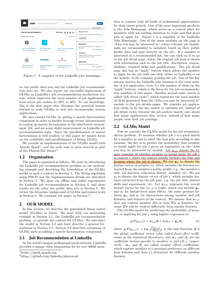
and the random e↵ects, respectively. An overview of the k-
th iteration of the block coordinate descent algorithm for
GLMix is given in Figure 2.
3.2.1
At iteration k of Algorithm 1, let sk denote the current
value of s = {sn}n2⌦. Let P denote the dimension of the
fixed e↵ect feature space, i.e., xn 2 RP , and Pr denote the
dimension of the feature space for random e↵ect r, i.e., zrn 2
RPr . And we use C to denote the overall dimension of the
feature space, that is:
Some Notations
C = P +Xr2R
PrNr,
(11)
where Nr denotes the number of random e↵ects of type r
(e.g., number of users). For the set of sample responses
y(⌦) = {yn}n2⌦, we use |⌦| to denote the size of ⌦, i.e.
the total number of training samples. We also let |R| be
the number of types of random e↵ects, and M be the num-
ber of computing nodes in the cluster. These numbers will
be used to compute and discuss the network I/O cost of our
proposed approach, which is usually one of the major bottle-
necks for an algorithm to scale up in a distributed computing
environment [27, 16]
3.2.2 Updating Fixed Effects
We consider the details of updating the fixed e↵ect b at
iteration k, following Equation (7). We start with preparing
the training data with both the feature set xn and the latest
score sk
n, and partition them into M nodes. This is identi-
fied as Superstep 1 in Figure 2. Given the training data,
numerous types of distributed algorithms can be applied to
learn b, such as [16, 6]. Here we adopt the all-reduce [1]
type of implementation for generalized linear models as in
MLlib [12]. First, the gradient of b for each sample n is com-
puted and aggregated from each node to the master node.
The master node computes the total gradient and updates b
using optimizers such as L-BFGS. This corresponds to Su-
perstep 2 in Figure 2. The new coe�cients bnew are then
broadcast back to each node together with bold to update
the score s as in Equation (9), in order to prepare for the
next e↵ect’s update. This phase corresponds to Superstep
3 in Figure 2. Since the main network communication here
is the transmission of b from the master node to the worker
nodes, the overall network communication cost for one iter-
ation of updating the fixed e↵ects is O(M P ). One trick we
found empirically useful is that it sometimes improves con-
vergence to update b multiple times before we update the
random e↵ects, for each iteration in Algorithm 1.
In summary, updating the fixed e↵ects consists of three
supersteps: (1) Preparing the training data with scores s.
(2) Updating the coe�cients b. (3) Updating the scores s.
3.2.3 Updating Random Effects
The main challenge in designing a scalable algorithm for
GLMix on data sets with a huge number of random e↵ects
is that the dimension of the random e↵ect coe�cient space
can potentially be as large as NrPr. Therefore, if we naively
apply the same approach as the one used in updating fixed
e↵ects, the network communication cost for updating the
random e↵ects for r becomes M NrPr. Given some data of
moderate size for example, if Nr = 106, Pr = 105 and a
cluster with M = 100, the network I/O cost amounts to
1013! As a result, the key to making the algorithm scalable
is to avoid communicating or broadcasting the random e↵ect
coe�cient across the computing nodes in the cluster.
Before the random e↵ect updating phase and as a prepro-
cessing step, for each random e↵ect r and ID l, we group
the feature vectors zrn to form a feature matrix Zrl, which
consists of all the zrn that satisfy i(r, n) = l. At iteration
k and for random e↵ect r, we shu✏e the current values of
s = {sk
n}n2⌦ using the same strategy, i.e. for ID l we group
sk
n to form a vector Sk
n that
satisfies i(r, n) = l. With the right partitioning strategies,
Sk
l can be made to collocate with the corresponding feature
matrix Zrl, to prepare the training data for updating the
random e↵ects r, using Equation (8). This step corresponds
to Superstep 4 in Figure 2. With the training data ready
for each ID l, any optimizer (e.g., L-BFGS) can be applied
again to solve the optimization problem locally, such that
the random e↵ects �rl can be learned in parallel without
l , which consists of all the sk
�
Figure 2: Overview of the kth iteration of the PBCD in BSP paradigm, with five supersteps highlighted in the blue boxes.
any additional network communication cost. Note that be-
cause both the coe�cients and data collocate in the same
node, the scores can be updated locally within the same
step, and this phase corresponds to Superstep 5 in Figure
2. Also note that during the whole process, the random ef-
fect coe�cients �rl live with the data and would never get
communicated through the network; only s would get shuf-
fled around the nodes through network I/O. As a result, the
overall network communication cost for one iteration of up-
dating one random e↵ects is O(|⌦|), and O(|R||⌦|) for |R|
random e↵ects.
Since the optimization problem in Equation (8) can be
solved locally, we have an opportunity to apply some tricks
that can further reduce the memory complexity C as defined
in Equation (11). Note that although the overall feature
space size is Pr for random e↵ect r, sometimes the under-
lying dimension of the feature matrix Zrl could be smaller
than Pr, due to the lack of support for certain features. For
example, a member who is a software engineer is unlikely
to be served jobs with the required skill ”medicine”. Hence
there will not be any data for the feature“job skill=medicine”
for this member’s random e↵ects, and in such a scenario, Zrl
would end up with an empty column. As a result, for each
random e↵ect r and ID l, we can condense Zrl by removing
all the empty columns and reindexing the features to form
a more compact feature matrix, which would also reduce
the size of random e↵ect coe�cients �rl and potentially im-
prove the overall e�ciency of solving the local optimization
problem in Equation (8). An example is shown in Figure 3,
where we compare the random e↵ect coe�cient size before
and after applying such a condensed data storage strategy
on a data set consisting of four months’ worth of LinkedIn’s
job recommendations. More details on the data set can be
found in Section 4.
In summary, the updating of random e↵ects consists of
two supersteps: (1) Prepare the training data with scores
s. (2) Update the random e↵ect coe�cients and also the
scores.
Summary
3.2.4
The overall I/O communication cost for our implementa-
tion for GLMix is O(M P + |R||⌦|). Since |R| is a small
constant (usually less than 5), the communication cost is
mainly bounded by the number of training instances |⌦|.
Figure 3: The member and job coe�cient size before and
after the reindexing and compression with the LinkedIn Job
Recommendation data set.
This is a significant improvement compared to the naive im-
plementation with a cost of O(M C), where C is defined in
(11), which could approach O(M Pr|⌦|) if we have a large
number of random e↵ects Nr that is of the same order as
the number of the training instances |⌦| (e.g., power law dis-
tribution). On the other hand, note that even with a large
scale data set with trillions of training samples, the size of s
is bounded to be a couple of terabytes. Given the recent ad-
vances in shu✏ing techniques [26], shu✏ing terabytes of data
is no longer a significant challenge. At the same time, since
the total number of random e↵ects Nr no longer depends
on the number of nodes in the cluster M , our algorithm has
the chance to scale linearly with the number of executors.
4. EXPERIMENTS OF LINKEDIN JOB REC-
OMMENDATION
In this section, we describe our experiments for the LinkedIn
job recommendation problem. Section 4.1 starts with the
o✏ine experimental results to compare several variations of
GLMix models with a couple of baselines for prediction ac-
curacy, and also experiments on scalability of GLMix in Sec-
tion 4.1. In Section 4.2 we share implementation details of
how we launched GLMix in LinkedIn’s production system.
We discuss the online A/B test results in Section 4.3.
4.1 Offline Experiments
4.1.1
All the methods used in the o✏ine experiments are im-
plemented using Apache Spark. In particular, the baseline
Setup
�
methods such as ridge regression, `2-regularized logistic re-
gression, matrix factorization with alternating least squares
are from Spark’s open source machine learning library ML-
lib. The experiments were conducted on a cluster consisting
of 135 nodes managed by Apache YARN 3. Each node has
24 Intel Xeon(R) CPU E5-2640 processors with 6 cores at
2.50GHz each, and every node has 250GB memory. In the
following experiments, Spark is running on top of YARN as a
client, and the memory for each Spark executor is configured
to 10GB, where each executor corresponds to a container
(e.g., a core of the node) in YARN.
4.1.2 Our Data
Our o✏ine experiments are conducted using a sample of
the four months’ worth of data (07/2015 - 11/2015) of mem-
ber’s interactions on the “Jobs You May Be Interested In”
module on the LinkedIn jobs homepage. The data include
500M samples with 5M members and 3M jobs. We split
the data by time into training (90%), validation (5%) and
test (5%).
Impressions that resulted in application clicks provide the
positive responses, and impressions that did not result in
application clicks provide the negative responses. Note that
the detail job views are not considered in this experiment,
since that is not the metric to optimize for. There are about
2K member features for qm, mostly extracted from public
member profiles, e.g. industry, job function, education his-
tory, skills, and so forth. There are also around 2K job fea-
tures for sj, e.g. the job title, key words in the description,
required skills and qualifications etc. We consider two types
of interactions among the member and job features: a) The
cosine-similarity of the member and job features in the same
domain, e.g. keywords in the summary of the member/job
profile, or the skills of the member / job requirement. There
are around 100 such cosine-similarity features, and we de-
note the feature vector as fc. b) The simple outer-product
of the member and job features. After applying standard
feature selection techniques we obtained 20K outer-product
features (denoted as fo).
4.1.3 Experiments of Performance
We consider the following models in our o✏ine experi-
ments (where g denotes the link function g(E[ymjt])):
• LR-Cosine: The baseline logistic regression model that
only includes the cosine-similarity features g = f0cb.
• LR-Full: The logistic regression model that includes all
global features, xmjt = {qm, sj, fc, fo}, g = x0mjtb.
• MF: A baseline matrix factorization model, g = x0mjtb+
u0mvj.
• GLMix-Member: The GLMix model which includes
only the member-level random e↵ects: g = x0mjtb +
s0j↵m.
• GLMix-Job: The GLMix model which includes only
the job-level random e↵ects: g = x0mjtb + q0m�j.
• GLMix-Full: The full GLMix model as described in
Equation (1).
• GLMix-Full+MF: An extension of GLMix which adds
an additional matrix factorization component, as in
Equation (4).
For each model listed above, we tried multiple values of
hyper-parameters for the priors (i.e. �b, �↵ and ��), picked
the ones with the best AUC performance on the validation
data, and then report their AUC on the test data in Table
1.
It is not surprising that adding the member and job
random e↵ects to the model dramatically improves the AUC
performance (0.723 for LR-Full vs 0.799 for GLMix-Full).
There are also two other interesting observations: a) GLMix-
Full significantly outperforms MF, which indicates that for
this data, using features to interact with member/job IDs
is more e↵ective than the interactions among member IDs
and job IDs. We believe this is due to the sparse structure
of the data and also because the features are very useful. b)
Adding matrix factorization to GLMix-Full provides very
little improvement in terms of AUC (0.799 to 0.801). This
indicates that GLMix already captures most signals of the
data, and adding matrix factorization for additional signals
in the residual is not e↵ective.
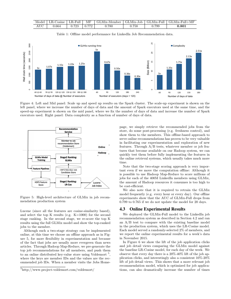
4.1.4 Experiments of Scalability
In this section, we study a) how GLMix scales up with the
increase of both data size and the number of Spark execu-
tors used, and b) how GLMix speeds up with the increase
of number of Spark executors, while fixing the data size. In
this experiment, the size of data is controlled by the number
of days used to collect the data, e.g., 60 days of the data is
about half of the size of 120 days of the data. The experi-
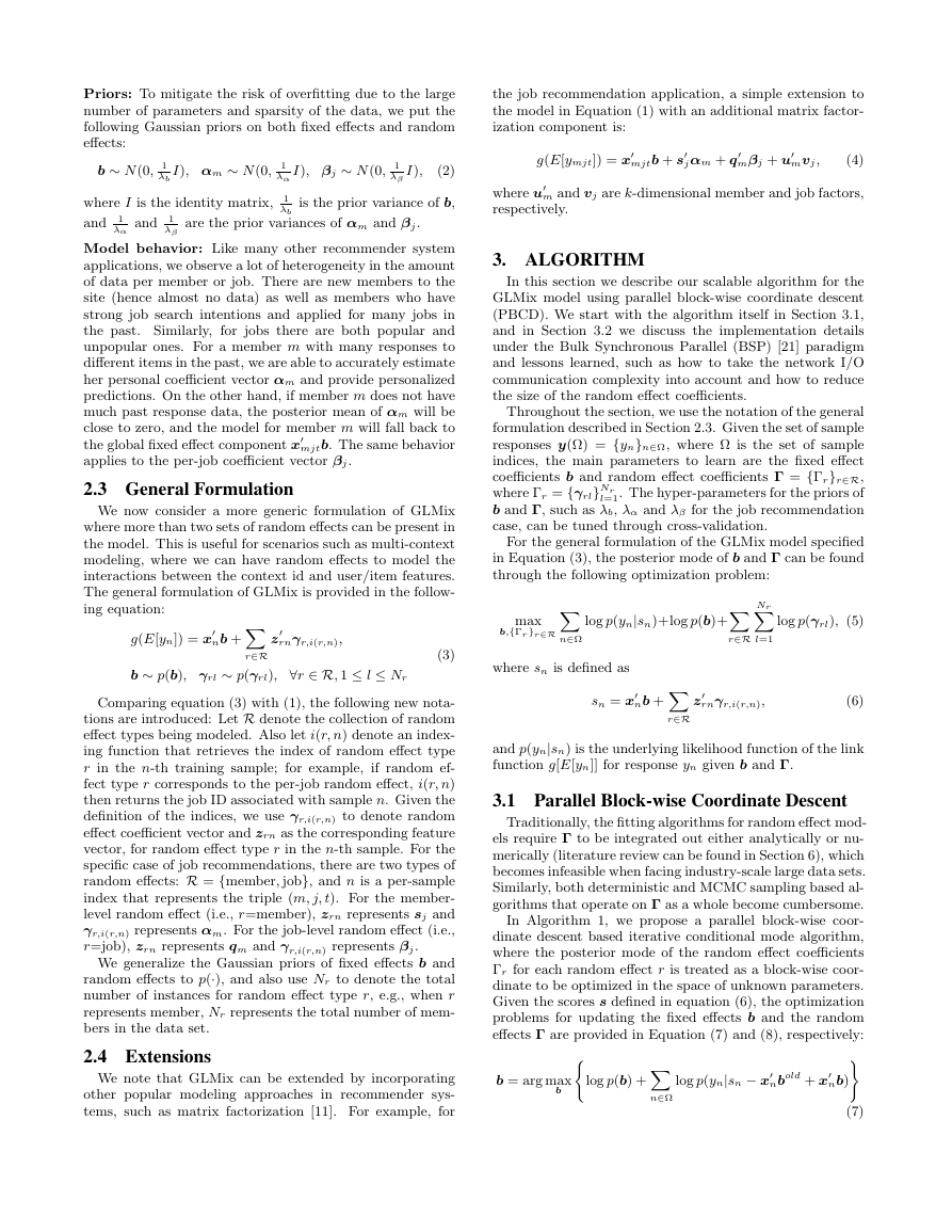
ment results can be found in Figure 4. In general, we find
that our proposed algorithm has good scalability properties,
and achieves roughly linear speed-up on the Spark cluster,
provided that the amount of data processed per executor
does not become so small that system overheads start to
dominate.
In Figure 4, we also provide the details on the change
of the data complexity C, as defined in Equation (11), as
the data size increases. We note that the scalability of our
implementation is quite robust to the increasing complexity
of the data set. If we had used the naive implementation
where the network I/O complexity is proportional to the
data complexity, it would have been much worse.
4.2 GLMix in Production System
LinkedIn operates one of the largest job recommendation
systems in the world, which serves relevant jobs to members
who visit the Job Homepage every day. For each member
visit, it is required that we rank millions of jobs using rel-
evance models and serve the top ranked ones in less than
a second. Apart from model training challenges, to pro-
ductionize a GLMix model with a huge number of features
and random e↵ects, the scoring and ranking become another
critical challenge to overcome.
Our approach to mitigate such a challenge is to have a
two-stage ranking strategy. In the first stage of the rank-
ing, we convert it to a search-like problem by leveraging the
open-source library Apache Lucene 4. In this stage, an in-
verted job index is built, where keys are the job features and
values are the corresponding job IDs. We run the baseline
model LR-Cosine in this stage, which works e�ciently with
3https://hadoop.apache.org
4https://lucene.apache.org/
�
Model LR-Cosine LR-Full MF GLMix-Member GLMix-Job GLMix-Full GLMix-Full+MF
AUC
0.801
0.664
0.723
0.772
0.780
0.758
0.799
Table 1: O✏ine model performance for LinkedIn Job Recommendation data.
0
0
0
3
0
0
5
2
0
0
0
2
0
0
5
1
0
0
0
1
0
0
5
0
GLMix running 4me
1x
1x
1.07x
1.15x
1.22x
1.25x
0.67x
0.50x
0.36x
0.30x
90 @ 90
60 @ 60
120 @ 120 150 @ 150 180 @ 180
Number of days of data @ Number of executors
60
90
120
180
240
Number of executors (days = 120)
5
2
0
2
5
1
0
1
5
0
)
n
o
i
l
l
i
B
(
e
z
S
i
1x
60
Complexity
2.51x
2.13x
1.75x
1.35x
120
90
Number of days of data
150
180
)
s
d
n
o
c
e
s
(
e
m
i
t
k
c
o
c
l
l
l
a
W
Figure 4: Left and Mid panel: Scale up and speed up results on the Spark cluster. The scale-up experiment is shown on the
left panel, where we increase the number of days of data and the amount of Spark executors used at the same time, and the
speed-up experiment is shown on the mid panel, where we fix the number of days of data and increase the number of Spark
executors used. Right panel: Data complexity as a function of number of days of data.
! "#$%%"&' ( ) $&*
+",- .#"*
/$#( .
- $. ) $/&0( &'( ) &
. $%+12( %&30( /$&
45( 6+$. ( /07&&
9 4:
.; *: $' "<*
=,( .&.&0*
+/( 0"8*! ( &2.&03**
9 4:
.; *
>"( /?,"*@.A"<.&"7*
89: 3&- $. ) $/&'( ) &
; 1%+<+10$&30( /$&
89: 3&: $10"/$&
30( /$&
+/( 0"1*! ( &2.&03**
4! 56$7*
B&<.&"*
C( ' $$A*
!"#$%$&
'( ) &*%+$, &
&
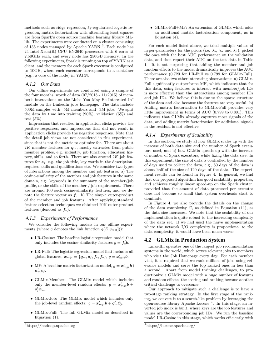
Figure 5: High-level architecture of GLMix in job recom-
mendation production system
Lucene (since all the features are cosine-similarity based),
and select the top K results (e.g. K=1000) for the second
stage ranking. In the second stage, we re-score the top K
results using the full GLMix model and show the top-ranked
jobs to the member.
Although such a two-stage strategy can be implemented
online, at this time we choose an o✏ine approach as in Fig-
ure 5, for more flexibility in experimentation and because
of the fact that jobs are usually more evergreen than news
articles. Through Hadoop Map-Reduce, we pre-generate the
top job recommendations for all members, and push them
to an online distributed key-value store using Voldemort 5,
where the keys are member IDs and the values are the rec-
ommended job IDs. When a member visits the Jobs Home-
5http://www.project-voldemort.com/voldemort/
page, we simply retrieve the recommended jobs from the
store, do some post-processing (e.g. freshness control), and
show them to the members. This o✏ine-based approach to
serve online recommendations has proven to be very valuable
in facilitating our experimentation and exploration of new
features. Through A/B tests, whatever member or job fea-
tures that become available on our Hadoop system, we can
quickly test them before fully implementing the features in
the online retrieval systems, which usually takes much more
time.
Note that the two-stage scoring approach is very impor-
tant even if we move the computation o✏ine: Although it
is possible to use Hadoop Map-Reduce to score millions of
jobs for each of the 400M LinkedIn members using GLMix,
the amount of Hadoop resources it consumes is too high to
be cost-e�cient.
We also note that it is required to retrain the GLMix
model frequently (e.g. every hour or every day). Our o✏ine
experiments show that the AUC of GLMix-Full drops from
0.799 to 0.765 if we do not update the model for 20 days.
4.3 Online Experimental Results
We deployed the GLMix-Full model to the LinkedIn job
recommendation system as described in Section 4.2 and ran
an A/B test to compare with the existing baseline model
in the production system, which uses the LR-Cosine model.
Each model served a randomly-selected 2% of members, and
we report the online experimental results for a week’s data
in November 2015.
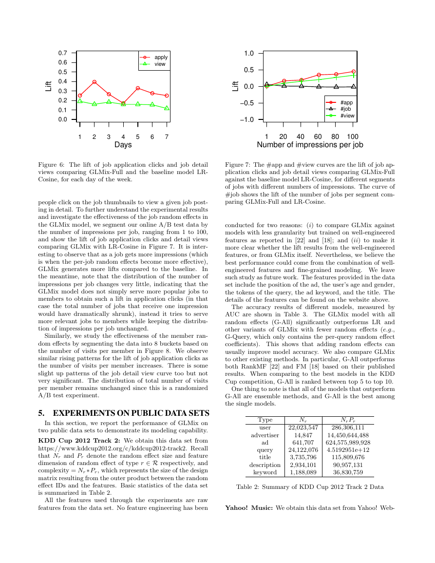
In Figure 6 we show the lift of the job application clicks
and job detail views comparing the GLMix model against
the baseline LR-Cosine model, for each day of the week. We
observe that every day there is a 20%-40% lift of the job ap-
plication clicks, and interestingly also a consistent 10%-20%
lift of job detail views. This shows that a more relevant job
recommendation model, which is optimized for job applica-
tions, can also dramatically increase the number of times
�
t
f
i
L
0.7
0.6
0.5
0.4
0.3
0.2
0.1
0.0
apply
view
1.0
0.5
t
f
i
L
0.0
−0.5
−1.0
#app
#job
#view
1
2
3
4
5
6
7
Days
1
20
40
60
80 100
Number of impressions per job
Figure 6: The lift of job application clicks and job detail
views comparing GLMix-Full and the baseline model LR-
Cosine, for each day of the week.
people click on the job thumbnails to view a given job post-
ing in detail. To further understand the experimental results
and investigate the e↵ectiveness of the job random e↵ects in
the GLMix model, we segment our online A/B test data by
the number of impressions per job, ranging from 1 to 100,
and show the lift of job application clicks and detail views
comparing GLMix with LR-Cosine in Figure 7. It is inter-
esting to observe that as a job gets more impressions (which
is when the per-job random e↵ects become more e↵ective),
GLMix generates more lifts compared to the baseline.
In
the meantime, note that the distribution of the number of
impressions per job changes very little, indicating that the
GLMix model does not simply serve more popular jobs to
members to obtain such a lift in application clicks (in that
case the total number of jobs that receive one impression
would have dramatically shrunk), instead it tries to serve
more relevant jobs to members while keeping the distribu-
tion of impressions per job unchanged.
Similarly, we study the e↵ectiveness of the member ran-
dom e↵ects by segmenting the data into 8 buckets based on
the number of visits per member in Figure 8. We observe
similar rising patterns for the lift of job application clicks as
the number of visits per member increases. There is some
slight up patterns of the job detail view curve too but not
very significant. The distribution of total number of visits
per member remains unchanged since this is a randomized
A/B test experiment.
5. EXPERIMENTS ON PUBLIC DATA SETS
In this section, we report the performance of GLMix on
two public data sets to demonstrate its modeling capability.
KDD Cup 2012 Track 2: We obtain this data set from
https://www.kddcup2012.org/c/kddcup2012-track2. Recall
that Nr and Pr denote the random e↵ect size and feature
dimension of random e↵ect of type r 2 R respectively, and
complexity = Nr⇤Pr, which represents the size of the design
matrix resulting from the outer product between the random
e↵ect IDs and the features. Basic statistics of the data set
is summarized in Table 2.
All the features used through the experiments are raw
features from the data set. No feature engineering has been
Figure 7: The #app and #view curves are the lift of job ap-
plication clicks and job detail views comparing GLMix-Full
against the baseline model LR-Cosine, for di↵erent segments
of jobs with di↵erent numbers of impressions. The curve of
#job shows the lift of the number of jobs per segment com-
paring GLMix-Full and LR-Cosine.
conducted for two reasons: (i) to compare GLMix against
models with less granularity but trained on well-engineered
features as reported in [22] and [18]; and (ii) to make it
more clear whether the lift results from the well-engineered
features, or from GLMix itself. Nevertheless, we believe the
best performance could come from the combination of well-
engineered features and fine-grained modeling. We leave
such study as future work. The features provided in the data
set include the position of the ad, the user’s age and gender,
the tokens of the query, the ad keyword, and the title. The
details of the features can be found on the website above.
The accuracy results of di↵erent models, measured by
AUC are shown in Table 3. The GLMix model with all
random e↵ects (G-All) significantly outperforms LR and
other variants of GLMix with fewer random e↵ects (e.g.,
G-Query, which only contains the per-query random e↵ect
coe�cients). This shows that adding random e↵ects can
usually improve model accuracy. We also compare GLMix
to other existing methods. In particular, G-All outperforms
both RankMF [22] and FM [18] based on their published
results. When comparing to the best models in the KDD
Cup competition, G-All is ranked between top 5 to top 10.
One thing to note is that all of the models that outperform
G-All are ensemble methods, and G-All is the best among
the single models.
Type
user
advertiser
ad
query
title
description
keyword
Nr
NrPr
22,023,547
286,306,111
14,847
641,707
24,122,076
3,735,796
2,934,101
1,188,089
14,450,644,488
624,575,989,928
4.5192951e+12
115,809,676
90,957,131
36,830,759
Table 2: Summary of KDD Cup 2012 Track 2 Data
Yahoo! Music: We obtain this data set from Yahoo! Web-
�




 2023年江西萍乡中考道德与法治真题及答案.doc
 2012年重庆南川中考生物真题及答案.doc
 2013年江西师范大学地理学综合及文艺理论基础考研真题.doc
 2020年四川甘孜小升初语文真题及答案I卷.doc
 2020年注册岩土工程师专业基础考试真题及答案.doc
 2023-2024学年福建省厦门市九年级上学期数学月考试题及答案.doc
 2021-2022学年辽宁省沈阳市大东区九年级上学期语文期末试题及答案.doc
 2022-2023学年北京东城区初三第一学期物理期末试卷及答案.doc
 2018上半年江西教师资格初中地理学科知识与教学能力真题及答案.doc
 2012年河北国家公务员申论考试真题及答案-省级.doc
 2020-2021学年江苏省扬州市江都区邵樊片九年级上学期数学第一次质量检测试题及答案.doc
 2022下半年黑龙江教师资格证中学综合素质真题及答案.doc