logo资料库

Introductory Time Series with R.pdf

第1页 / 共262页
第2页 / 共262页
第3页 / 共262页
第4页 / 共262页
第5页 / 共262页
第6页 / 共262页
第7页 / 共262页
第8页 / 共262页
资料共262页,剩余部分请下载后查看
Fotografía de página completa.pdf
00.pdf
Preface
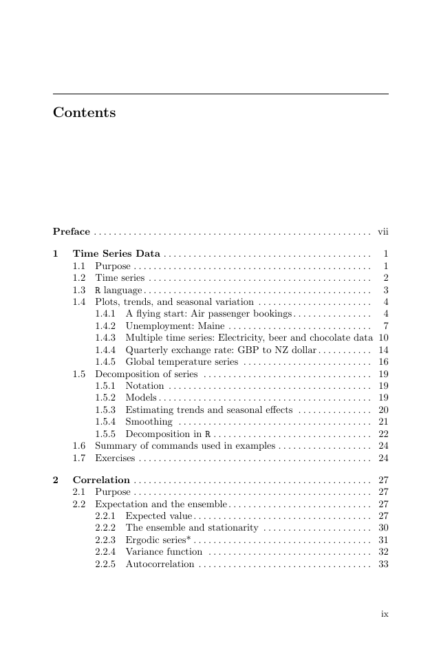
Contents
01.pdf
Time Series Data
Purpose
Time series
R language
Plots, trends, and seasonal variation
A flying start: Air passenger bookings
Unemployment: Maine
Multiple time series: Electricity, beer and chocolate data
Quarterly exchange rate: GBP to NZ dollar
Global temperature series
Decomposition of series
Notation
Models
Estimating trends and seasonal effects
Smoothing
Decomposition in R
Summary of commands used in examples
Exercises
02.pdf
Correlation
Purpose
Expectation and the ensemble
Expected value
The ensemble and stationarity
Ergodic series*
Variance function
Autocorrelation
The correlogram
General discussion
Example based on air passenger series
Example based on the Font Reservoir series
Covariance of sums of random variables
Summary of commands used in examples
Exercises
03.pdf
Forecasting Strategies
Purpose
Leading variables and associated variables
Marine coatings
Building approvals publication
Gas supply
Bass model
Background
Model definition
Interpretation of the Bass model*
Example
Exponential smoothing and the Holt-Winters method
Exponential smoothing
Holt-Winters method
Four-year-ahead forecasts for the air passenger data
Summary of commands used in examples
Exercises
04.pdf
Basic Stochastic Models
Purpose
White noise
Introduction
Definition
Simulation in R
Second-order properties and the correlogram
Fitting a white noise model
Random walks
Introduction
Definition
The backward shift operator
Random walk: Second-order properties
Derivation of second-order properties*
The difference operator
Simulation
Fitted models and diagnostic plots
Simulated random walk series
Exchange rate series
Random walk with drift
Autoregressive models
Definition
Stationary and non-stationary AR processes
Second-order properties of an AR(1) model
Derivation of second-order properties for an AR(1) process*
Correlogram of an AR(1) process
Partial autocorrelation
Simulation
Fitted models
Model fitted to simulated series
Exchange rate series: Fitted AR model
Global temperature series: Fitted AR model
Summary of R commands
Exercises
05.pdf
Regression
Purpose
Linear models
Definition
Stationarity
Simulation
Fitted models
Model fitted to simulated data
Model fitted to the temperature series (1970--2005)
Autocorrelation and the estimation of sample statistics*
Generalised least squares
GLS fit to simulated series
Confidence interval for the trend in the temperature series
Linear models with seasonal variables
Introduction
Additive seasonal indicator variables
Example: Seasonal model for the temperature series
Harmonic seasonal models
Simulation
Fit to simulated series
Harmonic model fitted to temperature series (1970--2005)
Logarithmic transformations
Introduction
Example using the air passenger series
Non-linear models
Introduction
Example of a simulated and fitted non-linear series
Forecasting from regression
Introduction
Prediction in R
Inverse transform and bias correction
Log-normal residual errors
Empirical correction factor for forecasting means
Example using the air passenger data
Summary of R commands
Exercises
06.pdf
Stationary Models
Purpose
Strictly stationary series
Moving average models
MA(q) process: Definition and properties
R examples: Correlogram and simulation
Fitted MA models
Model fitted to simulated series
Exchange rate series: Fitted MA model
Mixed models: The ARMA process
Definition
Derivation of second-order properties*
ARMA models: Empirical analysis
Simulation and fitting
Exchange rate series
Electricity production series
Wave tank data
Summary of R commands
Exercises
07.pdf
Non-stationary Models
Purpose
Non-seasonal ARIMA models
Differencing and the electricity series
Integrated model
Definition and examples
Simulation and fitting
IMA(1, 1) model fitted to the beer production series
Seasonal ARIMA models
Definition
Fitting procedure
ARCH models
S&P500 series
Modelling volatility: Definition of the ARCH model
Extensions and GARCH models
Simulation and fitted GARCH model
Fit to S&P500 series
Volatility in climate series
GARCH in forecasts and simulations
Summary of R commands
Exercises
08.pdf
Long-Memory Processes
Purpose
Fractional differencing
Fitting to simulated data
Assessing evidence of long-term dependence
Nile minima
Bellcore Ethernet data
Bank loan rate
Simulation
Summary of additional commands used
Exercises
09.pdf
Spectral Analysis
Purpose
Periodic signals
Sine waves
Unit of measurement of frequency
Spectrum
Fitting sine waves
Sample spectrum
Spectra of simulated series
White noise
AR(1): Positive coefficient
AR(1): Negative coefficient
AR(2)
Sampling interval and record length
Nyquist frequency
Record length
Applications
Wave tank data
Fault detection on electric motors
Measurement of vibration dose
Climatic indices
Bank loan rate
Discrete Fourier transform (DFT)*
The spectrum of a random process*
Discrete white noise
AR
Derivation of spectrum
Autoregressive spectrum estimation
Finer details
Leakage
Confidence intervals
Daniell windows
Padding
Tapering
Spectral analysis compared with wavelets
Summary of additional commands used
Exercises
10.pdf
System Identification
Purpose
Identifying the gain of a linear system
Linear system
Natural frequencies
Estimator of the gain function
Spectrum of an AR(p) process
Simulated single mode of vibration system
Ocean-going tugboat
Non-linearity
Exercises
11.pdf
Multivariate Models
Purpose
Spurious regression
Tests for unit roots
Cointegration
Definition
Exchange rate series
Bivariate and multivariate white noise
Vector autoregressive models
VAR model fitted to US economic series
Summary of R commands
Exercises
12.pdf
State Space Models
Purpose
Linear state space models
Dynamic linear model
Filtering*
Prediction*
Smoothing*
Fitting to simulated univariate time series
Random walk plus noise model
Regression model with time-varying coefficients
Fitting to univariate time series
Bivariate time series -- river salinity
Estimating the variance matrices
Discussion
Summary of additional commands used
Exercises
13.pdf
References
Index
Use R! Advisors: Robert Gentleman Kurt Hornik Giovanni Parmigiani For other titles published in this series, go to http://www.springer.com/series/6991
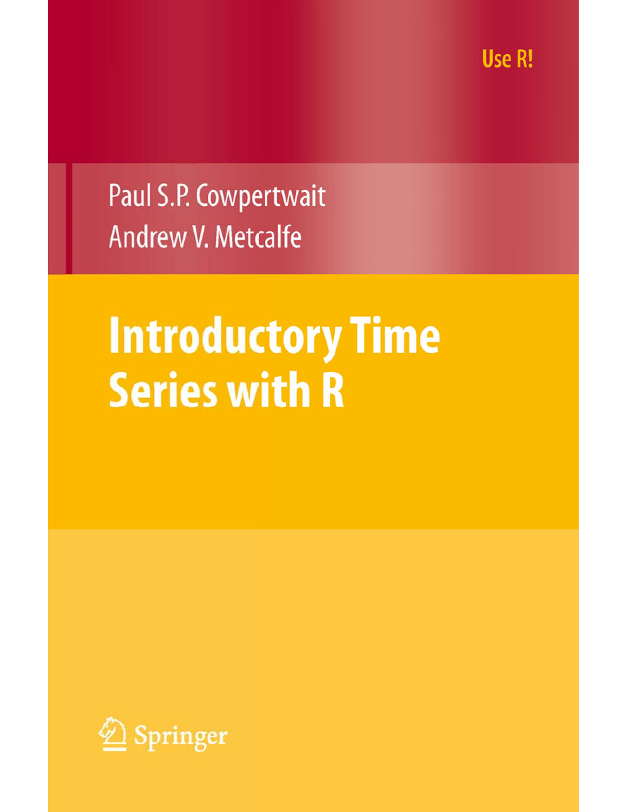
Paul S.P. Cowpertwait · Andrew V. Metcalfe Introductory Time Series with R 123
Paul S.P. Cowpertwait Inst. Information and Mathematical Sciences Massey University Auckland Albany Campus New Zealand p.s.cowpertwait@massey.ac.nz Andrew V. Metcalfe School of Mathematical Sciences University of Adelaide Adelaide SA 5005 Australia andrew.metcalfe@adelaide.edu.au Series Editors Robert Gentleman Program in Computational Biology Division of Public Health Sciences Fred Hutchinson Cancer Research Center 1100 Fairview Avenue, N. M2-B876 Seattle, Washington 98109 USA Kurt Hornik Department of Statistik and Mathematik Wirtschaftsuniversit¨at Wien Augasse 2-6 A-1090 Wien Austria Giovanni Parmigiani The Sidney Kimmel Comprehensive Cancer Center at Johns Hopkins University 550 North Broadway Baltimore, MD 21205-2011 USA ISBN 978-0-387-88697-8 DOI 10.1007/978-0-387-88698-5 Springer Dordrecht Heidelberg London New York e-ISBN 978-0-387-88698-5 Library of Congress Control Number: 2009928496 c⃝ Springer Science+Business Media, LLC 2009 All rights reserved. This work may not be translated or copied in whole or in part without the written permission of the publisher (Springer Science+Business Media, LLC, 233 Spring Street, New York, NY 10013, USA), except for brief excerpts in connection with reviews or scholarly analysis. Use in connection with any form of information storage and retrieval, electronic adaptation, computer software, or by similar or dissimilar methodology now known or hereafter developed is forbidden. The use in this publication of trade names, trademarks, service marks, and similar terms, even if they are not identified as such, is not to be taken as an expression of opinion as to whether or not they are subject to proprietary rights. Printed on acid-free paper Springer is part of Springer Science+Business Media (www.springer.com)
In memory of Ian Cowpertwait
Preface R has a command line interface that o↵ers considerable advantages over menu systems in terms of eciency and speed once the commands are known and the language understood. However, the command line system can be daunting for the first-time user, so there is a need for concise texts to enable the student or analyst to make progress with R in their area of study. This book aims to fulfil that need in the area of time series to enable the non-specialist to progress, at a fairly quick pace, to a level where they can confidently apply a range of time series methods to a variety of data sets. The book assumes the reader has a knowledge typical of a first-year university statistics course and is based around lecture notes from a range of time series courses that we have taught over the last twenty years. Some of this material has been delivered to post- graduate finance students during a concentrated six-week course and was well received, so a selection of the material could be mastered in a concentrated course, although in general it would be more suited to being spread over a complete semester. The book is based around practical applications and generally follows a similar format for each time series model being studied. First, there is an introductory motivational section that describes practical reasons why the model may be needed. Second, the model is described and defined in math- ematical notation. The model is then used to simulate synthetic data using R code that closely reflects the model definition and then fitted to the syn- thetic data to recover the underlying model parameters. Finally, the model is fitted to an example historical data set and appropriate diagnostic plots given. By using R, the whole procedure can be reproduced by the reader, and it is recommended that students work through most of the examples.1 Mathematical derivations are provided in separate frames and starred sec- 1 We used the R package Sweave to ensure that, in general, your code will produce the same output as ours. However, for stylistic reasons we sometimes edited our code; e.g., for the plots there will sometimes be minor di↵erences between those generated by the code in the text and those shown in the actual figures. vii
viii Preface tions and can be omitted by those wanting to progress quickly to practical applications. At the end of each chapter, a concise summary of the R com- mands that were used is given followed by exercises. All data sets used in the book, and solutions to the odd numbered exercises, are available on the website http://www.massey.ac.nz/⇠pscowper/ts. We thank John Kimmel of Springer and the anonymous referees for their helpful guidance and suggestions, Brian Webby for careful reading of the text and valuable comments, and John Xie for useful comments on an earlier draft. The Institute of Information and Mathematical Sciences at Massey Univer- sity and the School of Mathematical Sciences, University of Adelaide, are acknowledged for support and funding that made our collaboration possible. Paul thanks his wife, Sarah, for her continual encouragement and support during the writing of this book, and our son, Daniel, and daughters, Lydia and Louise, for the joy they bring to our lives. Andrew thanks Natalie for providing inspiration and her enthusiasm for the project. Paul Cowpertwait and Andrew Metcalfe Massey University, Auckland, New Zealand University of Adelaide, Australia December 2008
Contents Preface . . . . . . . . . . . . . . . . . . . . . . . . . . . . . . . . . . . . . . . . . . . . . . . . . . . . . . . . vii 1 1 Time Series Data . . . . . . . . . . . . . . . . . . . . . . . . . . . . . . . . . . . . . . . . . . 1 1.1 Purpose . . . . . . . . . . . . . . . . . . . . . . . . . . . . . . . . . . . . . . . . . . . . . . . . 2 1.2 Time series . . . . . . . . . . . . . . . . . . . . . . . . . . . . . . . . . . . . . . . . . . . . . 3 1.3 R language . . . . . . . . . . . . . . . . . . . . . . . . . . . . . . . . . . . . . . . . . . . . . . 4 1.4 Plots, trends, and seasonal variation . . . . . . . . . . . . . . . . . . . . . . . 4 1.4.1 A flying start: Air passenger bookings . . . . . . . . . . . . . . . . 1.4.2 Unemployment: Maine . . . . . . . . . . . . . . . . . . . . . . . . . . . . . 7 1.4.3 Multiple time series: Electricity, beer and chocolate data 10 1.4.4 Quarterly exchange rate: GBP to NZ dollar . . . . . . . . . . . 14 1.4.5 Global temperature series . . . . . . . . . . . . . . . . . . . . . . . . . . 16 1.5 Decomposition of series . . . . . . . . . . . . . . . . . . . . . . . . . . . . . . . . . . 19 1.5.1 Notation . . . . . . . . . . . . . . . . . . . . . . . . . . . . . . . . . . . . . . . . . 19 1.5.2 Models . . . . . . . . . . . . . . . . . . . . . . . . . . . . . . . . . . . . . . . . . . . 19 1.5.3 Estimating trends and seasonal e↵ects . . . . . . . . . . . . . . . 20 1.5.4 Smoothing . . . . . . . . . . . . . . . . . . . . . . . . . . . . . . . . . . . . . . . 21 1.5.5 Decomposition in R . . . . . . . . . . . . . . . . . . . . . . . . . . . . . . . . 22 1.6 Summary of commands used in examples . . . . . . . . . . . . . . . . . . . 24 1.7 Exercises . . . . . . . . . . . . . . . . . . . . . . . . . . . . . . . . . . . . . . . . . . . . . . . 24 2 Correlation . . . . . . . . . . . . . . . . . . . . . . . . . . . . . . . . . . . . . . . . . . . . . . . . 27 2.1 Purpose . . . . . . . . . . . . . . . . . . . . . . . . . . . . . . . . . . . . . . . . . . . . . . . . 27 2.2 Expectation and the ensemble . . . . . . . . . . . . . . . . . . . . . . . . . . . . . 27 2.2.1 Expected value . . . . . . . . . . . . . . . . . . . . . . . . . . . . . . . . . . . . 27 2.2.2 The ensemble and stationarity . . . . . . . . . . . . . . . . . . . . . . 30 2.2.3 Ergodic series* . . . . . . . . . . . . . . . . . . . . . . . . . . . . . . . . . . . . 31 2.2.4 Variance function . . . . . . . . . . . . . . . . . . . . . . . . . . . . . . . . . 32 2.2.5 Autocorrelation . . . . . . . . . . . . . . . . . . . . . . . . . . . . . . . . . . . 33 ix
分享到:
收藏