Foundations and Trends R in
Computer Graphics and Vision
Vol. 8, No. 2-3 (2012) 85–283
c 2014 J. Mairal, F. Bach and J. Ponce
DOI: 10.1561/0600000058
Sparse Modeling for Image and
Vision Processing
Julien Mairal
Inria 1
Francis Bach
Inria2
julien.mairal@inria.fr
francis.bach@inria.fr
Jean Ponce
Ecole Normale Supérieure3
jean.ponce@ens.fr
1LEAR team,
laboratoire Jean Kuntzmann, CNRS, Univ. Grenoble Alpes,
France.
2SIERRA team, département d’informatique de l’Ecole Normale Supérieure,
ENS/CNRS/Inria UMR 8548, France.
3WILLOW team, département d’informatique de l’Ecole Normale Supérieure,
ENS/CNRS/Inria UMR 8548, France.
�
Contents
1 A Short Introduction to Parsimony
1.1 Early concepts of parsimony in statistics . . . . . . . . . .
1.2 Wavelets in signal processing . . . . . . . . . . . . . . . .
1.3 Modern parsimony: the ℓ1-norm and other variants
. . . .
1.4 Dictionary learning . . . . . . . . . . . . . . . . . . . . . .
1.5 Compressed sensing and sparse recovery . . . . . . . . . .
1.6 Theoretical results about dictionary learning . . . . . . . .
2 Discovering the Structure of Natural Images
2.1 Pre-processing . . . . . . . . . . . . . . . . . . . . . . . .
2.2 Principal component analysis . . . . . . . . . . . . . . . .
2.3 Clustering or vector quantization . . . . . . . . . . . . . .
2.4 Dictionary learning . . . . . . . . . . . . . . . . . . . . . .
2.5 Structured dictionary learning . . . . . . . . . . . . . . . .
2.6 Other matrix factorization methods . . . . . . . . . . . . .
2.7 Discussion . . . . . . . . . . . . . . . . . . . . . . . . . .
3 Sparse Models for Image Processing
3.1
3.2
3.3
Image denoising . . . . . . . . . . . . . . . . . . . . . . .
Image inpainting . . . . . . . . . . . . . . . . . . . . . . .
Image demosaicking . . . . . . . . . . . . . . . . . . . . .
2
6
8
14
32
35
39
44
46
52
56
59
60
64
73
75
76
82
84
ii
�
Image up-scaling . . . . . . . . . . . . . . . . . . . . . . .
3.4
3.5
Inverting nonlinear local transformations . . . . . . . . . .
3.6 Video processing . . . . . . . . . . . . . . . . . . . . . . .
3.7 Face compression . . . . . . . . . . . . . . . . . . . . . .
. . . . . . . . . . . . .
3.8 Other patch modeling approaches
iii
87
92
94
96
99
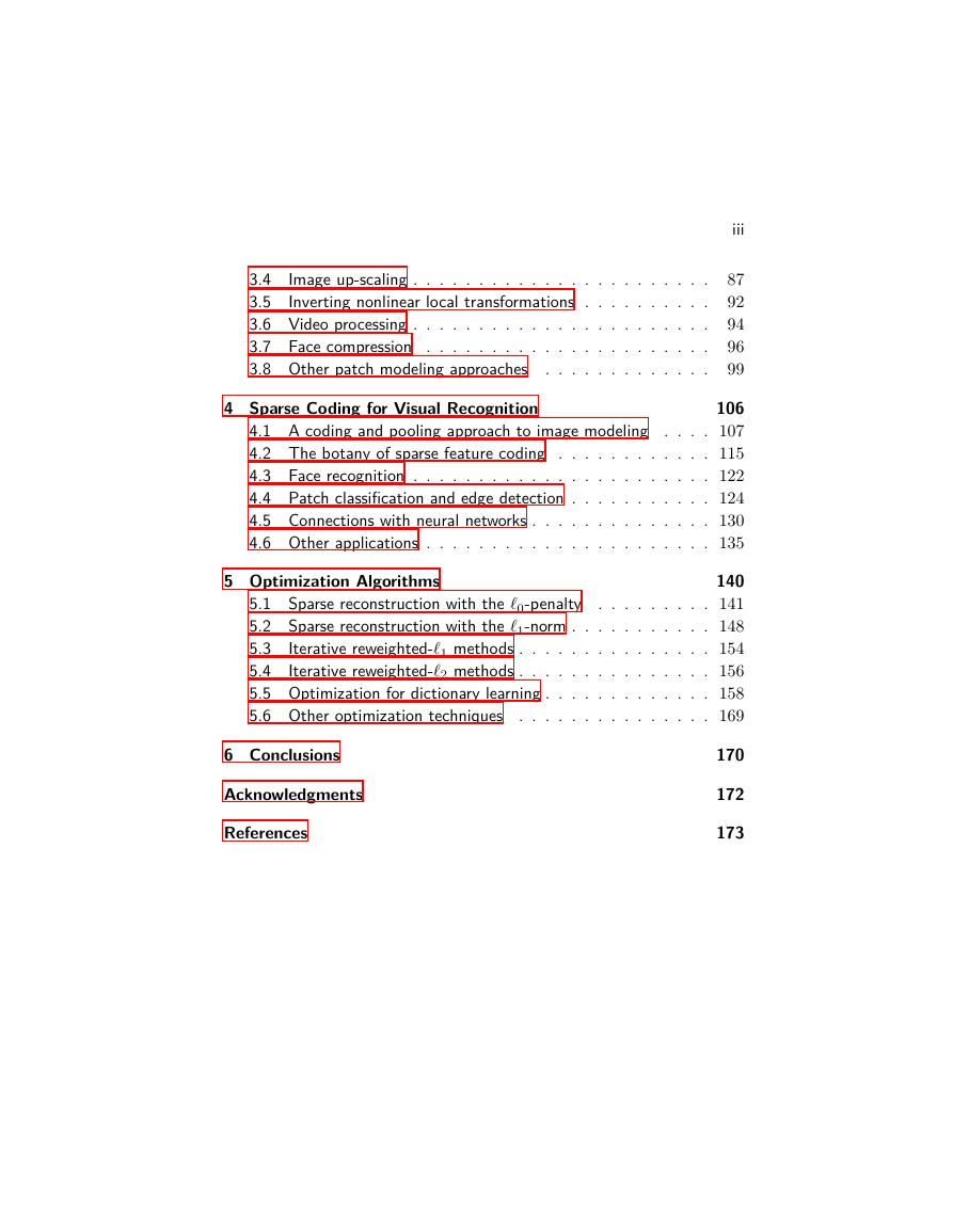
4 Sparse Coding for Visual Recognition
106
4.1 A coding and pooling approach to image modeling . . . . 107
4.2 The botany of sparse feature coding . . . . . . . . . . . . 115
4.3 Face recognition . . . . . . . . . . . . . . . . . . . . . . . 122
4.4 Patch classification and edge detection . . . . . . . . . . . 124
4.5 Connections with neural networks . . . . . . . . . . . . . . 130
4.6 Other applications . . . . . . . . . . . . . . . . . . . . . . 135
5 Optimization Algorithms
140
5.1 Sparse reconstruction with the ℓ0-penalty
. . . . . . . . . 141
5.2 Sparse reconstruction with the ℓ1-norm . . . . . . . . . . . 148
5.3
Iterative reweighted-ℓ1 methods . . . . . . . . . . . . . . . 154
5.4
Iterative reweighted-ℓ2 methods . . . . . . . . . . . . . . . 156
5.5 Optimization for dictionary learning . . . . . . . . . . . . . 158
5.6 Other optimization techniques
. . . . . . . . . . . . . . . 169
6 Conclusions
Acknowledgments
References
170
172
173
�
Abstract
In recent years, a large amount of multi-disciplinary research has been
conducted on sparse models and their applications. In statistics and
machine learning, the sparsity principle is used to perform model
selection—that is, automatically selecting a simple model among a large
collection of them. In signal processing, sparse coding consists of rep-
resenting data with linear combinations of a few dictionary elements.
Subsequently, the corresponding tools have been widely adopted by sev-
eral scientific communities such as neuroscience, bioinformatics, or com-
puter vision. The goal of this monograph is to offer a self-contained view
of sparse modeling for visual recognition and image processing. More
specifically, we focus on applications where the dictionary is learned
and adapted to data, yielding a compact representation that has been
successful in various contexts.
J. Mairal, F. Bach and J. Ponce. Sparse Modeling for Image and
Vision Processing. Foundations and Trends R in Computer Graphics and Vision,
vol. 8, no. 2-3, pp. 85–283, 2012.
DOI: 10.1561/0600000058.
�
1
A Short Introduction to Parsimony
In its most general definition, the principle of sparsity, or parsimony,
consists of representing some phenomenon with as few variables as
possible. It appears to be central to many research fields and is often
considered to be inspired from an early doctrine formulated by the
philosopher and theologian William of Ockham in the 14th century,
which essentially favors simple theories over more complex ones. Of
course, the link between Ockham and the tools presented in this mono-
graph is rather thin, and more modern views seem to appear later in
the beginning of the 20th century. Discussing the scientific method,
Wrinch and Jeffreys [1921] introduce indeed a simplicity principle re-
lated to parsimony as follows:
The existence of simple laws is, then, apparently, to be re-
garded as a quality of nature; and accordingly we may infer
that it is justifiable to prefer a simple law to a more complex
one that fits our observations slightly better.
Remarkably, Wrinch and Jeffreys [1921] further discuss statistical mod-
eling of physical observations and relate the concept of “simplicity” to
the number of learning parameters; as a matter of fact, this concept is
relatively close to the contemporary view of parsimony.
2
�
3
Subsequently, numerous tools have been developed by statisticians
to build models of physical phenomena with good predictive power.
Models are usually learned from observed data, and their generaliza-
tion performance is evaluated on test data. Among a collection of plau-
sible models, the simplest one is often preferred, and the number of
underlying parameters is used as a criterion to perform model selec-
tion [Mallows, 1964, 1966, Akaike, 1973, Hocking, 1976, Barron et al.,
1998, Rissanen, 1978, Schwarz, 1978, Tibshirani, 1996].
In signal processing, similar problems as in statistics arise, but a
different terminology is used. Observations, or data vectors, are called
“signals”, and data modeling appears to be a crucial step for perform-
ing various operations such as restoration, compression, or for solving
inverse problems. Here also, the sparsity principle plays an important
role and has been successful [Mallat and Zhang, 1993, Pati et al., 1993,
Donoho and Johnstone, 1994, Cotter et al., 1999, Chen et al., 1999,
Donoho, 2006, Candès et al., 2006]. Each signal is approximated by
a sparse linear combination of prototypes called dictionary elements,
resulting in simple and compact models.
However, statistics and signal processing remain two distinct fields
with different objectives and methodology; specifically, signals of-
ten come from the same data source, e.g., natural images, whereas
problems considered in statistics are unrelated to each other in gen-
eral. Then, a long series of works has been devoted to finding ap-
propriate dictionaries for signal classes of interest, leading to vari-
ous sorts of wavelets [Freeman and Adelson, 1991, Simoncelli et al.,
1992, Donoho, 1999, Candès and Donoho, 2002, Do and Vetterli, 2005,
Le Pennec and Mallat, 2005, Mallat, 2008]. Even though statistics and
signal processing have devised most of the methodology of sparse
modeling, the parsimony principle was also discovered independently
in other fields. To some extent,
it appears indeed in the work
of Markowitz [1952] about portfolio selection in finance, and also in
geophysics [Claerbout and Muir, 1973, Taylor et al., 1979].
In neuroscience, Olshausen and Field [1996, 1997] proposed a
significantly different approach to sparse modeling than previ-
ously established practices. Whereas classical techniques in signal
�
4
A Short Introduction to Parsimony
processing were using fixed off-the-shelf dictionaries, the method
of Olshausen and Field [1996, 1997] consists of learning it from train-
ing data. In a pioneer exploratory experiment, they demonstrated that
dictionary learning could easily discover underlying structures in nat-
ural image patches; later, their approach found numerous applica-
tions in many fields, notably in image and audio processing [Lewicki,
2002, Elad and Aharon, 2006, Mairal et al., 2009, Yang et al., 2010a]
and computer vision [Raina et al., 2007, Yang et al., 2009, Zeiler et al.,
2011, Mairal et al., 2012, Song et al., 2012, Castrodad and Sapiro,
2012, Elhamifar et al., 2012, Pokrass et al., 2013].
The goal of this monograph is to present basic tools of sparse mod-
eling and their applications to visual recognition and image processing.
We aim at offering a self-contained view combining pluri-disciplinary
methodology, practical advice, and a large review of the literature. Most
of the figures in the paper are produced with the software SPAMS1, and
the corresponding Matlab code will be provided on the first author’s
webpage.
The monograph is organized as follows: the current introductory
section is divided into several parts providing a simple historical view
of sparse estimation. In Section 1.1, we start with early concepts of
parsimony in statistics and information theory from the 70’s and 80’s.
We present the use of sparse estimation within the wavelet framework
in Section 1.2, which was essentially developed in the 90’s. Section 1.3
introduces the era of “modern parsimony”—that is, the ℓ1-norm and
its variants, which have been heavily used during the last two decades.
Section 1.4 is devoted to the dictionary learning formulation originally
introduced by Olshausen and Field [1996, 1997], which is a key com-
ponent of most applications presented later in this monograph. In Sec-
tions 1.5 and 1.6, we conclude our introductory tour with some theo-
retical aspects, such as the concept of “compressed sensing” and sparse
recovery that has attracted a large attention in recent years.
With all these parsimonious tools in hand, we discuss the use of
sparse coding and related sparse matrix factorization techniques for
discovering the underlying structure of natural image patches in Sec-
1available here http://spams-devel.gforge.inria.fr/.
�
5
tion 2 . Even though the task here is subjective and exploratory, it is
the first successful instance of dictionary learning; the insight gained
from these early experiments forms the basis of concrete applications
presented in subsequent sections.
Section 3 covers numerous applications of sparse models of natural
image patches in image processing, such as image denoising, super-
resolution, inpainting, or demosaicking. This section is concluded with
other related patch-modeling approaches.
Section 4 presents recent success of sparse models for visual recogni-
tion, such as codebook learning of visual descriptors, face recognition,
or more low-level tasks such as edge detection and classification of tex-
tures and digits. We conclude the section with other computer vision
applications such as visual tracking and data visualization.
Section 5 is devoted to optimization algorithms. It presents in a
concise way efficient algorithms for solving sparse decomposition and
dictionary learning problems.
We see our monograph as a good complement of other books and
monographs about sparse estimation, which offer different perspec-
tives, such as Mallat [2008], Elad [2010] in signal and image processing,
or Bach et al. [2012a] in optimization and machine learning. We also
put the emphasis on the structure of natural image patches learned with
dictionary learning, and thus present an alternative view to the book
of Hyvärinen et al. [2009], which is focused on independent component
analysis.
Notation.
In this monograph, vectors are denoted by bold lower-case
letters and matrices by upper-case ones. For instance, we consider in
the rest of this paragraph a vector x in Rn and a matrix X in Rm×n.
The columns of X are represented by indexed vectors x1, . . . , xn such
that we can write X = [x1, . . . , xn]. The i-th entry of x is denoted
by x[i], and the i-th entry of the j-th column of X is represented
by X[i, j]. For any subset g of {1, . . . , n}, we denote by x[g] the vec-
tor in R|g| that records the entries of x corresponding to indices in g.
For q ≥ 1, we define the ℓq-norm of x as kxkq , (Pn
i=1 |x[i]|q)1/q,
, limq→+∞ kxkq = maxi=1,...,n |x[i]|.
and the ℓ∞-norm as kxk∞
�





 2023年江西萍乡中考道德与法治真题及答案.doc
 2012年重庆南川中考生物真题及答案.doc
 2013年江西师范大学地理学综合及文艺理论基础考研真题.doc
 2020年四川甘孜小升初语文真题及答案I卷.doc
 2020年注册岩土工程师专业基础考试真题及答案.doc
 2023-2024学年福建省厦门市九年级上学期数学月考试题及答案.doc
 2021-2022学年辽宁省沈阳市大东区九年级上学期语文期末试题及答案.doc
 2022-2023学年北京东城区初三第一学期物理期末试卷及答案.doc
 2018上半年江西教师资格初中地理学科知识与教学能力真题及答案.doc
 2012年河北国家公务员申论考试真题及答案-省级.doc
 2020-2021学年江苏省扬州市江都区邵樊片九年级上学期数学第一次质量检测试题及答案.doc
 2022下半年黑龙江教师资格证中学综合素质真题及答案.doc