Cover
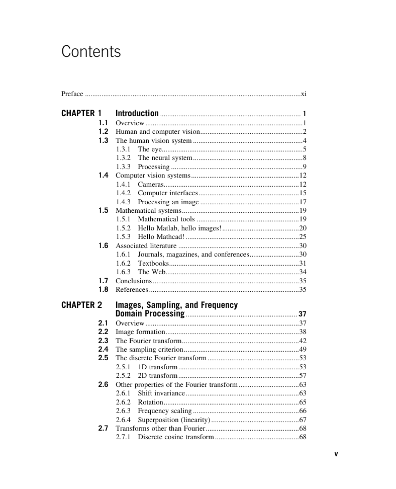
Contents
Preface
What is new in the third edition?
Why did we write this book?
The book and its support
In gratitude
Final message
Chapter 1 —
Introduction
1.1 Overview
1.2 Human and computer vision
1.3 The human vision system
1.3.1 The eye
1.3.2 The neural system
1.3.3 Processing
1.4 Computer vision systems
1.4.1 Cameras
1.4.2 Computer interfaces
1.4.3 Processing an image
1.5 Mathematical systems
1.5.1 Mathematical tools
1.5.2 Hello Matlab, hello images!
1.5.3 Hello Mathcad!
1.6 Associated literature
1.6.1 Journals, magazines, and conferences
1.6.2 Textbooks
1.6.3 The Web
1.7 Conclusions
1.8 References
Chapter 2 —
Images, sampling, and frequency domain processing
2.1 Overview
2.2 Image formation
2.3 The Fourier transform
2.4 The sampling criterion
2.5 The discrete Fourier transform
2.5.1 1D transform
2.5.2 2D transform
2.6 Other properties of the Fourier transform
2.6.1 Shift invariance
2.6.2 Rotation
2.6.3 Frequency scaling
2.6.4 Superposition (linearity)
2.7 Transforms other than Fourier
2.7.1 Discrete cosine transform
2.7.2 Discrete Hartley transform
2.7.3 Introductory wavelets
2.7.3.1 Gabor wavelet
2.7.3.2 Haar wavelet
2.7.4 Other transforms
2.8 Applications using frequency domain properties
2.9 Further reading
2.10 References
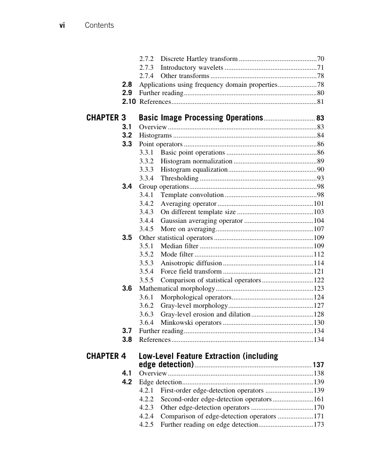
Chapter 3
— Basic image processing operations
3.1 Overview
3.2 Histograms
3.3 Point operators
3.3.1 Basic point operations
3.3.2 Histogram normalization
3.3.3 Histogram equalization
3.3.4 Thresholding
3.4 Group operations
3.4.1 Template convolution
3.4.2 Averaging operator
3.4.3 On different template size
3.4.4 Gaussian averaging operator
3.4.5 More on averaging
3.5 Other statistical operators
3.5.1 Median filter
3.5.2 Mode filter
3.5.3 Anisotropic diffusion
3.5.4 Force field transform
3.5.5 Comparison of statistical operators
3.6 Mathematical morphology
3.6.1 Morphological operators
3.6.2 Gray-level morphology
3.6.3 Gray-level erosion and dilation
3.6.4 Minkowski operators
3.7 Further reading
3.8 References
Chapter 4 —
Low-level feature extraction (including edge detection)
4.1 Overview
4.2 Edge detection
4.2.1 First-order edge-detection operators
4.2.1.1 Basic operators
4.2.1.2 Analysis of the basic operators
4.2.1.3 Prewitt edge-detection operator
4.2.1.4 Sobel edge-detection operator
4.2.1.5 The Canny edge detector
4.2.2 Second-order edge-detection operators
4.2.2.1 Motivation
4.2.2.2 Basic operators: the Laplacian
4.2.2.3 The Marr–Hildreth operator
4.2.3 Other edge-detection operators
4.2.4 Comparison of edge-detection operators
4.2.5 Further reading on edge detection
4.3 Phase congruency
4.4 Localized feature extraction
4.4.1 Detecting image curvature (corner extraction)
4.4.1.1 Definition of curvature
4.4.1.2 Computing differences in edge direction
4.4.1.3 Measuring curvature by changes in intensity (differentiation)
4.4.1.4 Moravec and Harris detectors
4.4.1.5 Further reading on curvature
4.4.2 Modern approaches: region/patch analysis
4.4.2.1 Scale invariant feature transform
4.4.2.2 Speeded up robust features
4.4.2.3 Saliency
4.4.2.4 Other techniques and performance issues
4.5 Describing image motion
4.5.1 Area-based approach
4.5.2 Differential approach
4.5.3 Further reading on optical flow
4.6 Further reading
4.7 References
Chapter 5 — High-level feature extraction: fixed shape matching
5.1 Overview
5.2 Thresholding and subtraction
5.3 Template matching
5.3.1 Definition
5.3.2 Fourier transform implementation
5.3.3 Discussion of template matching
5.4 Feature extraction by low-level features
5.4.1 Appearance-based approaches
5.4.1.1 Object detection by templates
5.4.1.2 Object detection by combinations of parts
5.4.2 Distribution-based descriptors
5.4.2.1 Description by interest points
5.4.2.2 Characterizing object appearance and shape
5.5 Hough transform
5.5.1 Overview
5.5.2 Lines
5.5.3 HT for circles
5.5.4 HT for ellipses
5.5.5 Parameter space decomposition
5.5.5.1 Parameter space reduction for lines
5.5.5.2 Parameter space reduction for circles
5.5.5.3 Parameter space reduction for ellipses
5.5.6 Generalized HT
5.5.6.1 Formal definition of the GHT
5.5.6.2 Polar definition
5.5.6.3 The GHT technique
5.5.6.4 Invariant GHT
5.5.7 Other extensions to the HT
5.6 Further reading
5.7 References
Chapter 6 —
High-level feature extraction: deformable shape analysis
6.1 Overview
6.2 Deformable shape analysis
6.2.1 Deformable templates
6.2.2 Parts-based shape analysis
6.3 Active contours (snakes)
6.3.1 Basics
6.3.2 The Greedy algorithm for snakes
6.3.3 Complete (Kass) snake implementation
6.3.4 Other snake approaches
6.3.5 Further snake developments
6.3.6 Geometric active contours (level-set-based approaches)
6.4 Shape skeletonization
6.4.1 Distance transforms
6.4.2 Symmetry
6.5 Flexible shape models—active shape and active appearance
6.6 Further reading
6.7 References
Chapter 7 —
Object description
7.1 Overview
7.2 Boundary descriptions
7.2.1 Boundary and region
7.2.2 Chain codes
7.2.3 Fourier descriptors
7.2.3.1 Basis of Fourier descriptors
7.2.3.2 Fourier expansion
7.2.3.3 Shift invariance
7.2.3.4 Discrete computation
7.2.3.5 Cumulative angular function
7.2.3.6 Elliptic Fourier descriptors
7.2.3.7 Invariance
7.3 Region descriptors
7.3.1 Basic region descriptors
7.3.2 Moments
7.3.2.1 Basic properties
7.3.2.2 Invariant moments
7.3.2.3 Zernike moments
7.3.2.4 Other moments
7.4 Further reading
7.5 References
Chapter 8
— Introduction to texture description, segmentation, and classification
8.1 Overview
8.2 What is texture?
8.3 Texture description
8.3.1 Performance requirements
8.3.2 Structural approaches
8.3.3 Statistical approaches
8.3.4 Combination approaches
8.3.5 Local binary patterns
8.3.6 Other approaches
8.4 Classification
8.4.1 Distance measures
8.4.2 The k-nearest neighbor rule
8.4.3 Other classification approaches
8.5 Segmentation
8.6 Further reading
8.7 References
Chapter 9 —
Moving object detection and description
9.1 Overview
9.2 Moving object detection
9.2.1 Basic approaches
9.2.1.1 Detection by subtracting the background
9.2.1.2 Improving quality by morphology
9.2.2 Modeling and adapting to the (static) background
9.2.3 Background segmentation by thresholding
9.2.4 Problems and advances
9.3 Tracking moving features
9.3.1 Tracking moving objects
9.3.2 Tracking by local search
9.3.3 Problems in tracking
9.3.4 Approaches to tracking
9.3.5 Meanshift and Camshift
9.3.5.1 Kernel-based density estimation
9.3.5.2 Meanshift tracking
Similarity function
Kernel profiles and shadow kernels
Gradient maximization
9.3.5.3 Camshift technique
9.3.6 Recent approaches
9.4 Moving feature extraction and description
9.4.1 Moving (biological) shape analysis
9.4.2 Detecting moving shapes by shape matching in image sequences
9.4.3 Moving shape description
9.5 Further reading
9.6 References
Chapter 10
— Appendix 1: Camera geometry fundamentals
10.1 Image geometry
10.2 Perspective camera
10.3 Perspective camera model
10.3.1 Homogeneous coordinates and projective geometry
10.3.1.1 Representation of a line and duality
10.3.1.2 Ideal points
10.3.1.3 Transformations in the projective space
10.3.2 Perspective camera model analysis
10.3.3 Parameters of the perspective camera model
10.4 Affine camera
10.4.1 Affine camera model
10.4.2 Affine camera model and the perspective projection
10.4.3 Parameters of the affine camera model
10.5 Weak perspective model
10.6 Example of camera models
10.7 Discussion
10.8 References
Chapter 11
— Appendix 2: Least squares analysis
11.1 The least squares criterion
11.2 Curve fitting by least squares
Chapter 12
— Appendix 3: Principal components analysis
12.1 Principal components analysis
12.2 Data
12.3 Covariance
12.4 Covariance matrix
12.5 Data transformation
12.6 Inverse transformation
12.7 Eigenproblem
12.8 Solving the eigenproblem
12.9 PCA method summary
12.10 Example
12.11 References
Chapter 13
— Appendix 4: Color images
13.1 Color images
13.2 Tristimulus theory
13.3 Color models
13.3.1 The colorimetric equation
13.3.2 Luminosity function
13.3.3 Perception based color models: the CIE RGB and CIE XYZ
13.3.3.1 CIE RGB color model: Wright–Guild data
13.3.3.2 CIE RGB color matching functions
13.3.3.3 CIE RGB chromaticity diagram and chromaticity coordinates
13.3.3.4 CIE XYZ color model
13.3.3.5 CIE XYZ color matching functions
13.3.3.6 XYZ chromaticity diagram
13.3.4 Uniform color spaces: CIE LUV and CIE LAB
13.3.5 Additive and subtractive color models: RGB and CMY
13.3.5.1 RGB and CMY
13.3.5.2 Transformation between RGB color models
13.3.5.3 Transformation between RGB and CMY color models
13.3.6 Luminance and chrominance color models: YUV, YIQ, and YCbCr
13.3.6.1 Luminance and gamma correction
13.3.6.2 Chrominance
13.3.6.3 Transformations between YUV, YIQ, and RGB color models
13.3.6.4 Color model for component video: YPbPr
13.3.6.5 Color model for digital video: YCbCr
13.3.7 Perceptual color models: HSV and HLS
13.3.7.1 The hexagonal model: HSV
13.3.7.2 The triangular model: HSI
13.3.8 More color models
13.4 References
Index




 2023年江西萍乡中考道德与法治真题及答案.doc
 2012年重庆南川中考生物真题及答案.doc
 2013年江西师范大学地理学综合及文艺理论基础考研真题.doc
 2020年四川甘孜小升初语文真题及答案I卷.doc
 2020年注册岩土工程师专业基础考试真题及答案.doc
 2023-2024学年福建省厦门市九年级上学期数学月考试题及答案.doc
 2021-2022学年辽宁省沈阳市大东区九年级上学期语文期末试题及答案.doc
 2022-2023学年北京东城区初三第一学期物理期末试卷及答案.doc
 2018上半年江西教师资格初中地理学科知识与教学能力真题及答案.doc
 2012年河北国家公务员申论考试真题及答案-省级.doc
 2020-2021学年江苏省扬州市江都区邵樊片九年级上学期数学第一次质量检测试题及答案.doc
 2022下半年黑龙江教师资格证中学综合素质真题及答案.doc