http://www.scirp.org/journal/jbise
J. Biomedical Science and Engineering,
2018, Vol. 11, (No. 6), pp: 144-157
Improved Protein Phosphorylation Site Prediction by a
New Combination of Feature Set and Feature Selection
Favorisen Rosyking Lumbanraja1, Ngoc Giang Nguyen1, Dau Phan1, Mohammad Reza Faisal1,
Bahriddin Abapihi1, Bedy Purnama1, Mera Kartika Delimayanti1, Mamoru Kubo2, Kenji Satou2
1Graduate School of Natural Science and Technology, Kanazawa University, Kanazawa, Japan; 2Institute of Science
and Engineering, Kanazawa University, Kanazawa, Japan
Correspondence to: Favorisen Rosyking Lumbanraja,
; Ngoc Giang Nguyen,
; Dau Phan,
; Mohammad Reza Faisal,
;
;
; Bedy Purnama,
; Mamoru Kubo,
Bahriddin Abapihi,
Mera Kartika Delimayanti,
Kenji Satou,
Keywords: Protein Phosphorylation, Phosphorylation Site Prediction, Sequence Feature, Feature Selection with
Grid Search
Received: May 27, 2018 Accepted: June 26, 2018 Published: June 29, 2018
Copyright © 2018 by authors and Scientific Research Publishing Inc.
This work is licensed under the Creative Commons Attribution International License (CC BY 4.0).
http://creativecommons.org/licenses/by/4.0/
;
Open Access
ABSTRACT
Phosphorylation of protein is an important post-translational modification that enables ac-
tivation of various enzymes and receptors included in signaling pathways. To reduce the
cost of identifying phosphorylation site by laborious experiments, computational prediction
of it has been actively studied. In this study, by adopting a new set of features and applying
feature selection by Random Forest with grid search before training by Support Vector
Machine, our method achieved better or comparable performance of phosphorylation site
prediction for two different data sets.
1. INTRODUCTION
Phosphorylation is one of the most important post-translational modifications (PTMs) in euka-
ryotes. This occurs when a phosphate group is added to a protein by a kinase. The addition of phosphate
group usually happens to Serine (S), Threonine, and Tyrosine (Y) [1]. It is also the common PTM, which
occur in eukaryotic cell [2]. Between 30% and 50% proteins of eukaryotic cell undergo phosphorylation
[3].
In the past, experimental approach such as mass spectrometry (MS/MS) [4] has been commonly used
to identify phosphorylation sites. However, implementing this approach has several disadvantages. Con-
ducting experiment to predict phosphorylation sites is considered expensive and requires intensive labor.
https://doi.org/10.4236/jbise.2018.116013
144
J. Biomedical Science and Engineering
�
In addition, it also requires adequate technique, skill, and specific equipment.
Instead, computational approach (in silico) is becoming more common because of new computer
technology development. These days, computers can process large number of data in a short time. This
makes prediction of phosphorylation sites using computational approach becoming more popular. Trost
and Kusalik provided summarization of various technique approach, data, and tools that can be applied to
predict phosphorylation site using computational approach [5].
In general, phosphorylation site prediction can be classified into two approaches: kinase-specific
phosphorylation site prediction and non-kinase-specific (general) phosphorylation site prediction. Ki-
nase-specific prediction approach requires both protein sequence and the type of kinase for phosphoryla-
tion to conduct prediction. The other approach is non-kinase-specific, which only requires protein se-
quence. Xue and Trost provided comparisons of these two approaches [5, 6]. The main disadvantage of
kinase-specific approach is that the publicly available information about the type of kinase is limited, espe-
cially for human kinase [7]. Therefore, non-kinase-specific approach is more popular to predict phospho-
rylation site [8].
There are various methods proposed for the prediction. For example, Blom used neural network
(NN) approach to predict eukaryotic protein phosphorylation site based on sequence and structure of
proteins [9]. Kim proposed a prediction method using support vector machine (SVM) [10].
In this paper, we propose a new prediction method for non-kinase-specific phosphorylation site. By
adopting a new combination of a classifier, features, and feature selection algorithm, we improved the
performance of prediction. We measured the result of feature selection and classification and compared it
with existing methods. We also tested our method with an independent data set and analysis of the classi-
fication result.
2. MATERIALS AND METHODS
2.1. Data Sets
In this work, we followed the preparation step done by Ismail [11]. The dataset we use were down-
loaded from the Phospho SVM website [12]. The phosphorylation site data set is P.ELM version 9 [13].
The data set contains phosphorylated sequences at the position of Serine (S), Threonine (T), and Tyrosine
(Y). These sequences were also checked for redundancy and sequences that had similarity more than 30%
were removed. Table 1 shows the number of sequences and number of sites for Serine, Threonine, and
Tyrosine, respectively.
We generated fixed-length protein sequences using window size 9, which have phospholyratable re-
sidues (Serine, Threonine, or Tyrosine) at the center of them. If the center residue of the sequence is
known as phosphorylated, the sequence is “positive”, otherwise “negative”. For positive and negative se-
quences, redundant ones were removed using skipredundant [14]. The parameters for redundancy remov-
al are as follows: acceptable threshold percentage of similarity was set to 0% - 20%, value for gap opening
penalty to 10, and gap extension penalty to 0.5. Table 2 shows the number of positive and negative se-
quences before and after removing redundant sequences for each residue.
The number of negative sequences after redundancy removal for Serine, Threonine, and Tyrosine re-
sidues are: 4771, 3343, and 898, respectively. We then randomly selected negative sequences for each resi-
due with the same number of negative sequences in the work of Ismail.
Using the same window size and method, we also generated sequences from PPA data set down-
loaded from the Phospho SVM website for conducting performance evaluation by independent data set.
PPA is a database for providing information of phosphorylation sites in Arabidopsis and a predictor for
plant-specific phosphorylation site [15]. After removal of redundant sequences, we randomly selected pos-
itive and negative sequences based on the work of Ismail. Table 3 shows number of positive and negative
phosphorylation sites for each amino acid. In order to make the data set well-balanced, the numbers of
positive and negative sequences were set to equal.
https://doi.org/10.4236/jbise.2018.116013
145
J. Biomedical Science and Engineering
�
Table 1. P.ELM data set of phosphorylation site from PhosphoSVM website.
Residue
Serine
Threonine
Tyrosine
Number of Sequence
Number of Sites
6635
3227
1392
20,964
5685
2163
Table 2. Number of sequences before and after removing redundant sequence for window size = 9.
Residue
Serine
Threonine
Tyrosine
Positive
Before
20,557
5596
1392
After
1554
707
267
Negative
1543
453
226
Table 3. PPA data set as the independent data set.
Residue
Serine
Threonine
Tyrosine
Number of positive/negative
sequences after redundancy removal
Number of positive/negative
sequences after selection
484/1830
132/1227
187/640
307/307
68/68
51/51
2.2. Methods
2.2.1. Feature Extraction
Using the fixed-length sequences, we conducted feature extraction to represent them as vectors of
numerical values. We used three different programs to extract features: PROFEAT (2016), PSI-BLAST,
and protr.
PROFEAT (2016) is a web server for extracting features from protein sequences [16]. We used it to
generate the following feaures: Amino Acid Composition, Dipeptide Composition, Normalized Mo-
reau-Broto Autocorrelation Descriptor, Moran Autocorrelation Descriptor, Moran Autocorrelation De-
scriptor, Geary Autocorrelation Descriptor, Composition, Transition, Distribution Descriptor, Amphi-
philic Pseudo-Amino Acid Composition, and Total Amino Acid Properties. For Position Specific Scoring
Matrix (PSSM) features, we used PSI-BLAST [17]. In addition, an R package called protrwas used to pro-
duce the following features: BLOSUM and PAM Matrices for the 20 Amino Acid, Amino Acid Properties
Based Scales Descriptor (Protein Fingerprint), Scales-based Descriptor derived by Principal Components
Analysis, Scales-based Descriptor derived by Multidimensional Scaling, Conjoint Triad Descriptors, and
Sequence-Order-Coupling Number [18]. Details of these features are described below. Except three fea-
tures (CTD, SOCN, QSO), most of the features are not used in Ismail’s work.
Amino Acid Composition (AAC)
Amino Acid Composition is defined as the fraction of each amino acid in a protein sequence [19]. For
all 20 amino acids, the fraction is calculated using this equation.
fraction of
aa =
i
total of number of amino acid type
i
total number of amino acid in protein sequence
(1)
https://doi.org/10.4236/jbise.2018.116013
146
J. Biomedical Science and Engineering
�
where i is a spesific type of amino acid
Dipeptide Composition (DPC)
Dipeptide Composition generates 400 fixed-length numeric information based on the input protein
sequences. It encapsulates information about the fraction of amino acid as well as their local order. It is
calculated using Equation (2):
fraction of
( )
dep i =
total of number of
( )
dep i
total number of all posible dipeptide
(2)
where dep(i) is one dipeptide i of 400 dipeptides.
Normalized Moreau-Broto Autocorrelation Descriptors (NMB)
Before we calculate Normalized Moreau-Broto Autocorrelation, we must define Moreau-Broto Au-
tocorrelation. It can be define using Equation (3):
(
)
AC d
(3)
where Pi and Pi+d are the amino acid property at position i and i + d, respectively. Normalized Mo-
reau-Broto Autocorrelation is defined using Equation (4) [20]:
(
)
AC d
N d
−
(4)
(
ATS d
PP
i
i d
+
=
)
= ∑
N d
−
i
1
=
When we usePROFEAT, the value of nlag should be lower than the size of the sequence. Since the
where d = 1, 2, 3, ∙∙∙, 30.
window size is 9, we setnlag = 8.
Moran Autocorrelation Descriptors (MORAN)
Moran Autocorrelation can be calculated using Equation (5):
)
i d
+
P
−
(
1
−
N d
(
I d
)
=
N d
−
i
1
=
∑
∑
1
N
−
)(
P P P
i
(
)
P P
i
−
2
N
i
1
=
,
d
=
1,2,3,
(5)
,30
where P is the avarege of Pi. In the use of PROFEAT, we setnlag = 8.
Geary Autocorrelation Descriptors (GEARY)
Geary Autocorrelation can be defined using Equation (6):
)
−
(
2
,
)
)
2
)
(
2
(
1
d
=
−
=
i d
+
N
N
i
1
=
∑
∑
,30
N d
−
i
1
=
(
C d
1,2,3,
P P
i
P P
i
1
N d
−
1
−
In the use of PROFEAT, we setnlag = 8.
Composition, Transition, Distribution (CTD)
Composition, Transition, Distribution represent the amino acid distribution patterns of a certain
structural or physicochemical property from a protein sequences. These features are calculated as follows:
the protein sequence is transformed into a sequence of a specific physicochemical or structural properties
of residue. Twenty amino acids are divided into three groups [20, 21].
(6)
Composition (C), Transition (T), and Distribution (D) are then calculated for a given attribute to de-
scribe the global percent composition if the three groups of amino acids in a protein, the percent frequen-
cies with which the attribute changes its index along the entire length of the protein, and the distribution
pattern of attribute along the sequence, respectively.
Sequence-Order-Coupling Number (SOCN)
Sequence-Order-Coupling Number can be used to represent amino acid distribution pattern of a spe-
cific physicochemical property along a protein sequence. The dth rank of sequence-order-coupling num-
https://doi.org/10.4236/jbise.2018.116013
147
J. Biomedical Science and Engineering
�
ber can be calculated using Equation (7):
=
∑
N d
−
i
1
=
(
2
)
τ
d
(7)
where di,i+d is the distance between two amino acid at position i and i + d. In the use of protr, we also set-
nlag = 8.
Quasi-Sequence-Order Descriptors (QSO)
Quasi-Sequence-Order Descriptors can be calculated using Sequence-Order-Coupling Number. For
each amino acid type, the type-1 Quasi-Sequence-Order Descriptors is calculated using Equation (8):
1,2,
,30
i i d
,
+
3,
=
d
d
,
X
r
=
∑
20
r
1
=
f
r
f
+
r
w
∑
30
τ
d
d
1
=
,
r
=
1,2,3,
(8)
,20
where fr is the normalized occurrence of amino acid type i and w is the weighting factor, w = 0.1. The
type-2 Quasi-Sequence-Order Descriptors is calculated using Equation (9):
w
τ
d
+
20
−
∑
w
X
d
=
,
r
=
21,22,23,
(9)
,50
r
f
∑
30
τ
d
d
1
=
20
r
1
=
In the use of PROFEAT, we setnlag = 8.
Amphiphilic Pseudo-Amino Acid Composition(APAAC)
Before we calculate Amphiphilic Pseudo-Amino Acid Composition, we must define Pseudo-Amino
Acid Composition (PAAC) [22]. First, three variables are generated from the original hydrophobicity val-
0M i of 20 amino acids (i = 1, 2, 3, ∙∙∙,
ues
20).
, and side chain masses
, hydrophilicity values
( )
2H i
( )
1H i
( )
0
0
( )
H i
1
=
( )
H i
2
=
( )
M i
=
( )
H i
0
1
−
∑
20
i
1
=
∑
20
i
( )
H i
0
1
−
∑
20
( )
H i
0
2
−
∑
20
i
1
=
∑
20
i
( )
H i
0
2
−
∑
20
( )
0
H i
1
20
( )
0
H i
1
20
20
i
1
=
( )
0
H i
2
20
( )
0
H i
2
20
20
i
1
=
2
2
(10)
(11)
M
0
( )
i
20
0
M
( )
i
20
0
M
( )
i
−
∑
20
i
1
=
∑
20
i
0
M
( )
i
∑
20
i
1
=
20
(12)
2
Then, a correlation function can generated as:
(
θ
R R
i
,
j
)
=
1
3
+
{
1
1
)
−
(
H R
i
(
H R
(
M R M R
−
(
)
i
j
j
2
2
)
) }
+
(
H R
i
2
)
−
(
H R
2
j
2
)
(13)
https://doi.org/10.4236/jbise.2018.116013
148
J. Biomedical Science and Engineering
�
From which, sequence order-correlated factors are defined as:
)
,
λ λ
<
θ
λ
R R
i
i
(
N
λ
−
θ
i
1
=
=
(
,
+
1
− ∑
λ
N
N
)
(14)
where λ is parameter. Let fi be the normalized frequency of 20 amino acids in the protein sequence, a set of
20 + λ descriptors called the PAAC can be defined using Equation (15):
, when 1
≤ ≤
u
20
u
f
+
X
u
=
X
u
=
∑
20
i
1
=
f w λ
∑
λθ
i
j
1
=
20
∑
i
1
=
w
θ
u
20
f w λ
∑
+
θ
i
λ
j
1
=
−
, when 20 1
+ ≤ ≤
u
20
+
λ
(15)
where w = 0.05. From Equation (10) and Equation (11), the hydrophobicity and hydrophilicity correlation
can be define as:
H
1
i
,
j
=
H i H j H
;
,
( )
( )
1
1
2
i
,
j
=
( )
H i H j
( )
,
2
2
(16)
Then, sequence order factor can be define using Equation (17):
2
i i
,
∑
λ
Finally, APAAC can be calculated using Equation (18):
N
λ
−
H
i
1
=
N
λ
−
H
i
1
=
τ
1
2
λ
−
τ
2
λ
1
−
1
−
∑
λ
;
λ
1
i i
,
N
N
=
=
+
, where
λ
+
λ
<
2
(17)
f
u
+
∑
2
λτ
j
j
1
=
, when 1
≤
u
≤
20
p
u
=
p
u
=
∑
20
i
1
=
i
f
20
∑
i
1
=
w
τ
u
∑
+
f
i
, when 20 1
+ ≤ ≤
u
20
+
λ
(18)
2
λ
τ
j
j
1
=
In the use of PROFEAT, we set weight factor = 0.05 and lamda = 8.
Total Amino Acid Properties (AAP)
Total Amino Acid Properties for a specific physicochemical property i is defined using Equation (19):
(19)
represents the property i of amino acid Rj that is normalized between 0 and 1.N is the length
= ∑
N
P=
j
1
no
p
( )
tot i
1
N
rm
i
j
where
of the protein sequence.
normP
i
j
normP
i
j
is calculated using Equation (20):
i
p
−
min
i
p
−
min
i
jp is the original amino acid property i for residue j.
ip
where
max
maximum values of the original amino acid property i, respectively.
p
i
p
max
P
norm
=
i
j
i
j
(20)
and
ip
min
are the minimum and the
Position Specific Scoring Matrix (PSSM)
PSSM features were generated using PSI-BLAST against a local database generated from the phos-
phorylation data set.
BLOSUM and PAM Matrices for the 20 Amino Acid (BLOSUM)
In the use of protr, we setk = 5, lag = 3, and Matrix type = AABLOSUM45.
Amino Acid Properties Based Scales Descriptor (Protein Fingerprint) (ProtFP)
In the use of protr, we set pc = 5, lag = 5, index vector for Amino Acid Index = (160:165, 258:296).
Scales-based Descriptor derived by Principal Components Analysis (SCALES)
In the use of protr, we set pc = 7, lag = 5, properties matrix = AA index (7:26).
Scales-based Descriptor derived by Multidimensional Scaling (MDDSCALES)
In the use of protr, we set lag = 8.
https://doi.org/10.4236/jbise.2018.116013
149
J. Biomedical Science and Engineering
�
Conjoint Triad Descriptors (CTriad) [22]
2.2.2. Feature Selection
Random Forest was introduced by Breiman [23]. Random Forest method works as a collection of
large number of decision trees randomly generated and not correlated to each other. This method is wide-
lyapplied to classification problems.
In Random Forest, Gini impurity index (GII) is used to measure feature importance. GII represents
how often randomly chosen element from the data set would be classified incorrectly if it was randomly
classified based on the distribution of classes in the subset. We use Gini Index to rank important features
that can be used for the classification algorithm.
In [11], Ismail also attempted the same feature selection and top 100 features were selected. In con-
trast, we conducted grid search to find the best set of selected features.
2.2.3. Classification
Vapnik [24] proposed support vector machine (SVM) as a classification method. It is a popular clas-
sifier widely applied to various problems including phosphorylation site prediction. SVM produces an op-
timal hyperplane separation between the classes. Here, optimal means finding the maximum margin
around the separating hyperplane. In this work, we adopted Gaussian (also known as radial basis function)
kernel for SVM.
2.2.4. Evaluation
10-fold cross-validation was repeated 10 times to measure the average performance of the P.ELM da-
ta. To measure the performance for the PPA data set, which is used for the independent data set,
leave-one-out cross-validation (LOOCV) was conducted.
The metricsused to measure the classification performance are: Accuracy, Sensitivity, Specificity, F1
score, and Matthew’s Correlation Coefficient (MCC). These metrics are defined in the following equations:
Accuracy
=
TP TN FP FN
+
+
(21)
TP TN
+
+
TP
TP FN
+
TN
+
TP
TN FP
Sensitiviy
=
(22)
Specificity
=
(23)
TP FP FN
F1score
(
(
+
×
)
TP FP
= ×
2
+
)
TP TN
−
)
TP FN
×
×
+
(
(
(24)
+
)
FP FN
)
TN FP
(25)
TN FN
×
+
×
+
(
)
MCC
=
(
where TP, TN, FP, and FN are the abbreviation for true positive, true negative, false positive, and false
negative. In this work, Area under the ROC curve (AUC) is also measured.
3. RESULT AND DISCUSSION
3.1. P.ELM Data Set
3.1.1. Feature Selection
Gini impurity index (GII) in Random Forest was used to measure the importance of the features. For
P.ELM data set, we conducted 10-fold cross validation repeated 10 times. For each fold in each iteration,
we generate a list of important features based on the training data. Then we average the value GII of each
features from the 100 list features we generated before. To give insight of which features that effects the
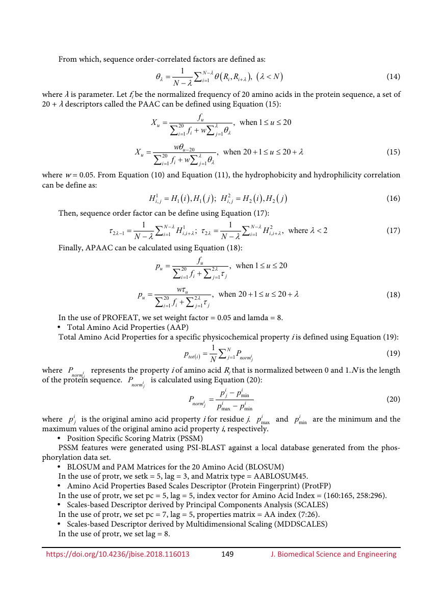
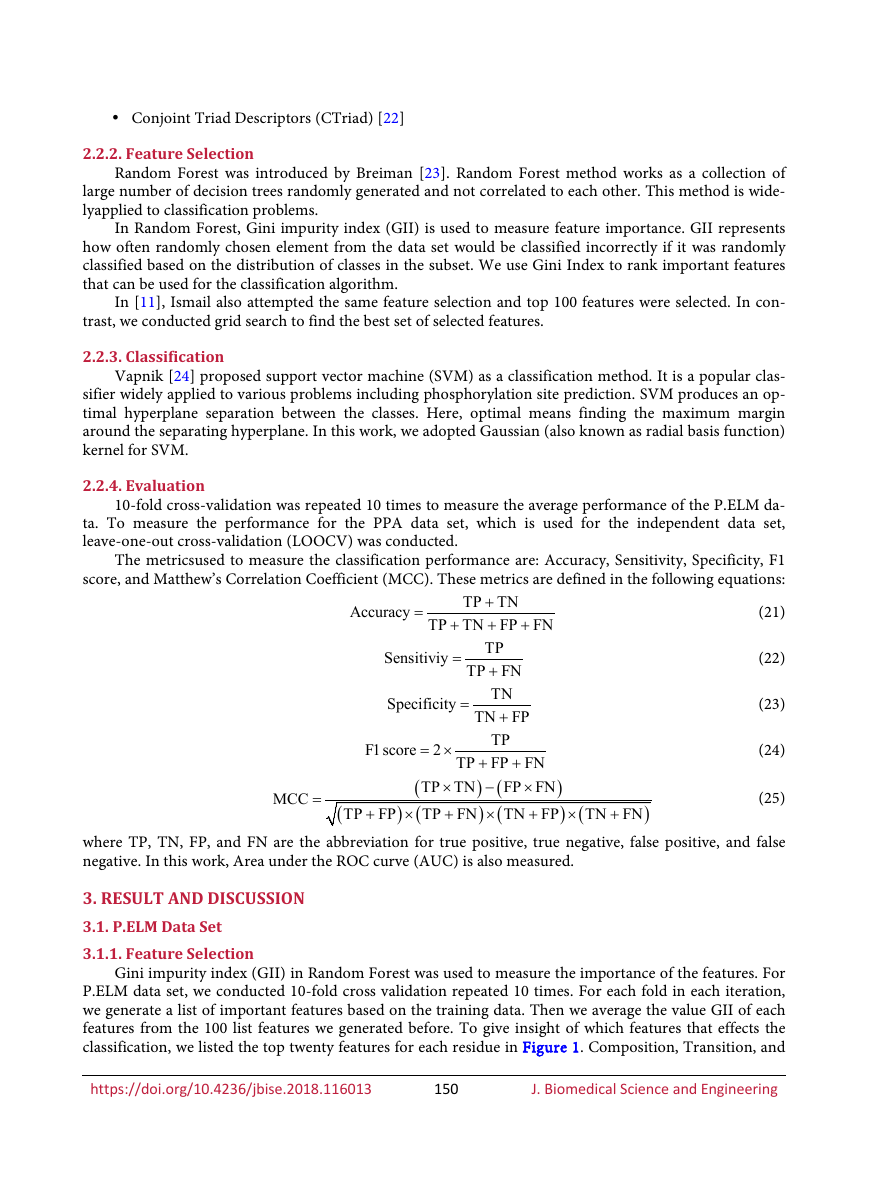
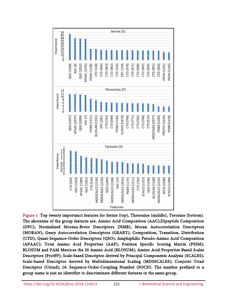
classification, we listed the top twenty features for each residue in Figure 1. Composition, Transition, and
https://doi.org/10.4236/jbise.2018.116013
150
J. Biomedical Science and Engineering
�
Figure 1. Top twenty importanct features for Serine (top), Threonine (middle), Tyrosine (bottom).
The akronims of the group features are: Amino Acid Composition (AAC);Dipeptide Composition
(DPC); Normalized Moreau-Broto Descriptors (NMB); Moran Autocorrelation Descriptors
(MORAN); Geary Autocorrelation Descriptors (GEARY); Composition, Transition, Distribution
(CTD); Quasi-Sequence-Order Descriptors (QSO); Amphiphilic Pseudo-Amino Acid Composition
(APAAC); Total Amino Acid Properties (AAP); Position Specific Scoring Matrix (PSSM);
BLOSUM and PAM Matrices the 20 Amino Acid (BLOSUM); Amino Acid Properties Based Scales
Descriptors (ProtFP); Scale-based Descriptor derived by Principal Components Analysis (SCALES);
Scale-based Descriptor derived by Multidimensional Scaling (MDSSCALES); Conjoint Triad
Descriptor (Ctriad); 16: Sequence-Order-Coupling Number (SOCN). The number prefixed to a
group name is just an identifier to descriminate different features in the same group.
https://doi.org/10.4236/jbise.2018.116013
151
J. Biomedical Science and Engineering
�



 2023年江西萍乡中考道德与法治真题及答案.doc
 2012年重庆南川中考生物真题及答案.doc
 2013年江西师范大学地理学综合及文艺理论基础考研真题.doc
 2020年四川甘孜小升初语文真题及答案I卷.doc
 2020年注册岩土工程师专业基础考试真题及答案.doc
 2023-2024学年福建省厦门市九年级上学期数学月考试题及答案.doc
 2021-2022学年辽宁省沈阳市大东区九年级上学期语文期末试题及答案.doc
 2022-2023学年北京东城区初三第一学期物理期末试卷及答案.doc
 2018上半年江西教师资格初中地理学科知识与教学能力真题及答案.doc
 2012年河北国家公务员申论考试真题及答案-省级.doc
 2020-2021学年江苏省扬州市江都区邵樊片九年级上学期数学第一次质量检测试题及答案.doc
 2022下半年黑龙江教师资格证中学综合素质真题及答案.doc