Efficient Processing of Deep Neural Networks:
A Tutorial and Survey
Vivienne Sze, Senior Member, IEEE, Yu-Hsin Chen, Student Member, IEEE, Tien-Ju Yang, Student
Member, IEEE, Joel Emer, Fellow, IEEE
1
7
1
0
2
r
a
M
7
2
]
V
C
.
s
c
[
1
v
9
3
0
9
0
.
3
0
7
1
:
v
i
X
r
a
Abstract—Deep neural networks (DNNs) are currently widely
used for many artificial intelligence (AI) applications including
computer vision, speech recognition, and robotics. While DNNs
deliver state-of-the-art accuracy on many AI tasks, it comes at the
cost of high computational complexity. Accordingly, techniques
that enable efficient processing of deep neural network to improve
energy-efficiency and throughput without sacrificing performance
accuracy or increasing hardware cost are critical to enabling the
wide deployment of DNNs in AI systems.
This article aims to provide a comprehensive tutorial and
survey about the recent advances towards the goal of enabling
efficient processing of DNNs. Specifically,
it will provide an
overview of DNNs, discuss various platforms and architectures
that support DNNs, and highlight key trends in recent efficient
processing techniques that reduce the computation cost of DNNs
either solely via hardware design changes or via joint hardware
design and network algorithm changes. It will also summarize
various development resources that can enable researchers and
practitioners to quickly get started on DNN design, and highlight
important benchmarking metrics and design considerations that
should be used for evaluating the rapidly growing number
of DNN hardware designs, optionally including algorithmic co-
design, being proposed in academia and industry.
The reader will take away the following concepts from this
article: understand the key design considerations for DNNs;
be able to evaluate different DNN hardware implementations
with benchmarks and comparison metrics; understand trade-
offs between various architectures and platforms; be able to
evaluate the utility of various DNN design techniques for efficient
processing; and understand of recent implementation trends and
opportunities.
I. INTRODUCTION
Deep neural networks (DNNs) are currently the foundation
for many modern AI applications [1]. Since the breakthrough
application of DNNs to speech recognition [2] and image
recognition [3], the number of applications that use DNNs
has exploded. These DNNs are employed in a myriad of
applications from self-driving cars [4], to detecting cancer [5]
to playing complex games [6]. In many of these domains,
DNNs are now able to exceed human accuracy. The superior
performance of DNNs comes from its ability to extract high-
level features from raw sensory data after using statistical
learning over a large amount of data to obtain an effective
V. Sze, Y.-H. Chen and T.-J. Yang are with the Department of Electrical
Engineering and Computer Science, Massachusetts Institute of Technol-
ogy, Cambridge, MA 02139 USA. (e-mail: sze@mit.edu; yhchen@mit.edu,
tjy@mit.edu)
J. S. Emer is with the Department of Electrical Engineering and Computer
Science, Massachusetts Institute of Technology, Cambridge, MA 02139 USA,
and also with Nvidia Corporation, Westford, MA 01886 USA. (e-mail:
jsemer@mit.edu)
representation of an input space. This is different from earlier
approaches that use hand-crafted features or rules designed by
experts.
The superior accuracy of DNNs, however, comes at the
cost of high computational complexity. While general-purpose
compute engines, especially graphics processing units (GPUs),
have been the mainstay for much DNN processing, increasingly
there is interest in providing more specialized acceleration of
the DNN computations. This article aims to provide an overview
of DNNs, the various tools for understanding their behavior,
and techniques being explored to efficiently accelerate their
computations.
This paper is organized as follows:
• Section II provides background on the context of why
DNNs are important, their history and applications.
• Section III gives an overview of the basic components of
DNNs and popular DNN models currently in use.
• Section IV describe the various resources used for DNN
research and development.
• Section V describes the various hardware platforms used
to process DNN and the various optimizations to improve
throughput and energy without impacting performance
accuracy (i.e., produces bit-wise identical results).
• Section VI discusses how mixed-signal circuits and new
memory technologies can be used for near-data processing
to address the challenging data movement that dominates
throughput and energy consumption of DNNs.
• Section VII describes various joint algorithm and hardware
optimizations that can be performed on DNNs to improve
both throughput and energy while trying to minimize
impact on performance accuracy.
• Section VIII describes the key metrics that should be
considered when comparing various DNNs designs.
II. BACKGROUND ON DEEP NEURAL NETWORKS (DNN)
In this section, we describe the position of deep neural
networks (DNNs) in the context of AI in general and some
of the concepts that motivated its development. We will also
present a brief chronology of the major steps in its history, and
some current domains to which it is being applied.
A. Artificial Intelligence and DNNs
Deep neural networks, also referred to as deep learning, are
part of the broad field of artificial intelligence (AI), which is
the science and engineering of creating intelligent machines
that have the ability to achieve goals like humans do, according
�
2
brain.
A key characteristic of the synapse is that it can scale the
value crossing it. That scaling factor can be referred to as a
weight, and the way the brain is believed to learn is through
changes to the weights associated with the synapses. Thus,
different weights result in different responses to an input. Note
that learning is the adjustment of the weights in response to
a learning stimulus, while the organization (what might be
thought of as the program) of the brain does not change. This
characteristic makes the brain an excellent inspiration for a
machine-learning-style algorithm.
Within the brain-inspired computing paradigm there is a
subarea called spiking computing. In this subarea, inspiration
is taken from the fact that the communication on the dendrites
and axons are spike-like pulses and that the information being
conveyed is not just based on a spike’s amplitude. Instead,
it also depends on the time the pulse arrives and that the
computation that happens in the neuron is a function of not just
a single value but the width of pulse and the timing relationship
between different pulses. An example of a project that was
inspired by the spiking of the brain is the IBM TrueNorth [7].
In contrast to spiking computing, another subarea of brain-
inspired computing is called neural networks, which is the
focus of this article.
B. Neural Networks and Deep Neural Networks (DNNs)
Neural networks take their inspiration from the notion that
a neuron’s computation involves a weighted sum of the input
values. These weighted sums correspond to the value scaling
performed by the synapses and the combining of those values
in the neuron. Furthermore, the neuron doesn’t just output that
weighted sum, since the computation associated with a cascade
of neurons would then be a simple linear algebra operation.
Instead there is a functional operation within the neuron that
is performed on the combined inputs. This operation appears
to be a non-linear function that causes a neuron to generate
an output only if the inputs cross some threshold. Thus by
analogy, neural networks apply a non-linear function to the
weighted sum of the input values. We look at what some of
those non-linear functions are later.
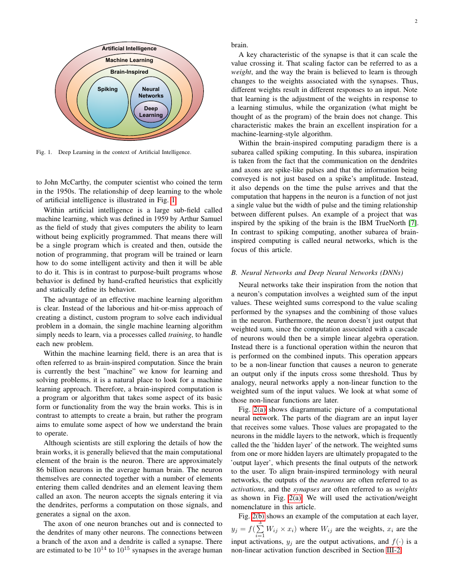
Fig. 2(a) shows diagrammatic picture of a computational
neural network. The parts of the diagram are an input layer
that receives some values. Those values are propagated to the
neurons in the middle layers to the network, which is frequently
called the the ’hidden layer’ of the network. The weighted sums
from one or more hidden layers are ultimately propagated to the
’output layer’, which presents the final outputs of the network
to the user. To align brain-inspired terminology with neural
networks, the outputs of the neurons are often referred to as
activations, and the synapses are often referred to as weights
as shown in Fig. 2(a). We will used the activation/weight
nomenclature in this article.
3
Fig. 2(b) shows an example of the computation at each layer,
Wij × xi) where Wij are the weights, xi are the
yj = f (
input activations, yj are the output activations, and f (·) is a
non-linear activation function described in Section III-2.
i=1
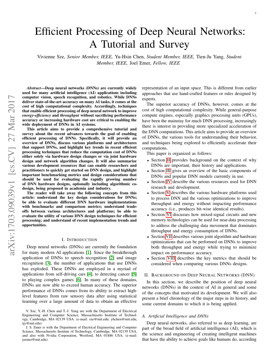
Fig. 1. Deep Learning in the context of Artificial Intelligence.
to John McCarthy, the computer scientist who coined the term
in the 1950s. The relationship of deep learning to the whole
of artificial intelligence is illustrated in Fig. 1.
Within artificial
intelligence is a large sub-field called
machine learning, which was defined in 1959 by Arthur Samuel
as the field of study that gives computers the ability to learn
without being explicitly programmed. That means there will
be a single program which is created and then, outside the
notion of programming, that program will be trained or learn
how to do some intelligent activity and then it will be able
to do it. This is in contrast to purpose-built programs whose
behavior is defined by hand-crafted heuristics that explicitly
and statically define its behavior.
The advantage of an effective machine learning algorithm
is clear. Instead of the laborious and hit-or-miss approach of
creating a distinct, custom program to solve each individual
problem in a domain, the single machine learning algorithm
simply needs to learn, via a processes called training, to handle
each new problem.
Within the machine learning field, there is an area that is
often referred to as brain-inspired computation. Since the brain
is currently the best ”machine” we know for learning and
solving problems, it is a natural place to look for a machine
learning approach. Therefore, a brain-inspired computation is
a program or algorithm that takes some aspect of its basic
form or functionality from the way the brain works. This is in
contrast to attempts to create a brain, but rather the program
aims to emulate some aspect of how we understand the brain
to operate.
Although scientists are still exploring the details of how the
brain works, it is generally believed that the main computational
element of the brain is the neuron. There are approximately
86 billion neurons in the average human brain. The neuron
themselves are connected together with a number of elements
entering them called dendrites and an element leaving them
called an axon. The neuron accepts the signals entering it via
the dendrites, performs a computation on those signals, and
generates a signal on the axon.
The axon of one neuron branches out and is connected to
the dendrites of many other neurons. The connections between
a branch of the axon and a dendrite is called a synapse. There
are estimated to be 1014 to 1015 synapses in the average human
Artificial Intelligence Machine Learning Brain-Inspired Spiking Neural Networks Deep Learning �
3
the DNN is a vectors of scores, one for each object class; the
class with the highest score indicates the most likely class of
object in the image. The overarching goal for training a DNN
is to determine how to set the weights to maximize the score
of the correct class (as given from the labeled training data),
and minimize the scores of the other incorrect classes. The
gap between the ideal correct scores and the scores computed
by the DNN based on its current weights is referred to as the
loss (L). Thus the goal of training DNNs is to find a set of
weights to minimize the average loss over a large dataset.
The weights (wij) are updated using a hill-climbing opti-
mization process called gradient decent. A multiple of the
gradient of the loss relative to each weight, which is the partial
derivative of the loss for the weight, is used to update the
weight (i.e., updated wt+1
, where α is called
the learning rate). Note that this gradient indicates how the
weights should change in order to reduce the loss. The process
is repeated iteratively to reduce the overall loss.
ij − α dL
ij = wt
dwij
The gradient itself is efficiently computed through a process
called back-propagation where the impact of the loss is passed
backwards through the network to compute how the loss is
affected by each weight.
This back-propagation computation is, in fact, very similar
in form to the computation used for inference. Thus, techniques
for efficiently performing inference can sometimes be useful for
performing training. It is important to note, however, that due
to the gradients use for hill-climbing, the precision requirement
for training is higher than inference. Thus many of the reduced
precision techniques discussed in Section VII are limited to
inference only.
A variety of techniques are used to improve the efficiency
and robustness of training. For example, often the loss from
multiple sets of input data, i.e., a batch, are collected before a
weight update is performed; this helps to speed up and stabilize
the training process.
There are multiple ways to train the weights. The most
common approach, described above, is called supervised learn-
ing, where all the training samples are labelled. Unsupervised
learning is another approach where all the training samples
are not labeled and essentially the goal is to find structure or
clusters in the data. Semi-supervised learning falls in between
the two approaches where only a small subset of the training
data is labeled (e.g., use unlabeled data to define the cluster
boundaries, and use the small amount of labeled data to label
the clusters). Finally, reinforcement learning can be used to
train a DNN to be a policy network such that given an input, it
can output a decision on what action to take next and receive
the corresponding reward; the process of training this network
is to make decisions that maximize the received rewards (i.e.,
a reward function), and the training process must balance
exploration (trying new actions) and exploitation (using actions
that are known to give high rewards).
Another commonly used approach to determine weights
is fine-tuning, where previously-trained weights are used as
initialization and then weights are adjusted for a new dataset
(e.g., transfer learning) or for a new constraint (e.g., reduced
precision). This results in faster training as compared to starting
from a random initialization, and can sometime result in better
(a) Neurons and synapses
(b) Compute weighted sum for each layer
(c) Feedforward versus feedback (re-
current) networks
(d) Fully connected versus sparse
Fig. 2. Simple Neural Network Example (Figure adopted from [8].)
Within the domain of neural networks, we have an area
called deep learning. The original neural networks had very
few layers in the network. In deep networks there are many
more layers in the network. Networks today have five to more
than a thousand of layers.
A current interpretation of the activity for vision applications
in the many layers of these deep networks is that after entering
all the pixels of an image into the first layer of the network,
the weighted sums of that layer can be interpreted as the
representing the presence of different low-level features in
the image. At subsequent layers these features are combined
into a measure of the likely presence of higher and higher
level features, e.g. lines are combined into shapes, which are
further combined into sets of shapes. And finally, given all
this information the network provides a probability that these
high-level features comprise a particular object.
Although this area is popularly called deep learning, the
fundamental computation consists of various forms of deeply
layered neural nets. Therefore, we will generally use the
terminology deep neural networks (DNNs) in this article.
C. Inference versus Training
Since DNNs are an instance of a machine learning algorithm,
the basic program does not change as it learns to perform
its given tasks. In the specific case of DNNs, this learning
involves determining the value of the weights in the network.
This learning is referred to as training the network.
Once trained, the program can be run performing the network
computation using the weights determined by the training. This
operation of using the network to perform it task is referred
to as inference.
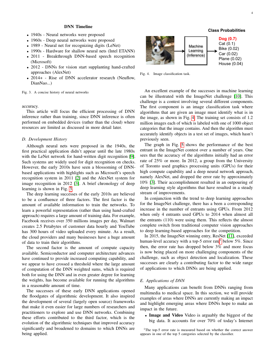
In this section, we will use image classification, as shown
in Fig. 4, as a driving example for training a DNN. When we
evaluate a DNN, we give an input image and the output of
Neurons (activations) Synapses (weights) X1 X2 X3 Y1 Y2 Y3 Y4 W11 W34 L1 Input Neurons (e.g. image pixels) Layer 1 L1 Output Neurons a.k.a. Activations Layer 2 L2 Output Neurons Feed Forward Recurrent Fully-Connected Sparsely-Connected �
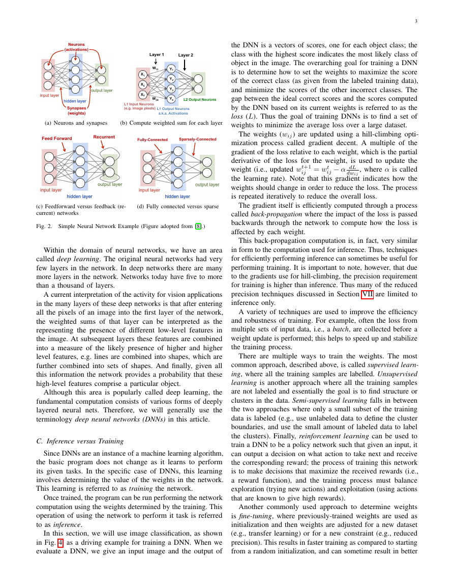
DNN Timeline
4
• 1940s - Neural networks were proposed
• 1960s - Deep neural networks were proposed
• 1989 - Neural net for recognizing digits (LeNet)
• 1990s - Hardware for shallow neural nets (Intel ETANN)
• 2011 - Breakthrough DNN-based speech recognition
(Microsoft)
• 2012 - DNNs for vision start supplanting hand-crafted
• 2014+ - Rise of DNN accelerator research (Neuflow,
approaches (AlexNet)
DianNao...)
Fig. 4.
Image classification task.
Fig. 3. A concise history of neural networks
accuracy.
This article will focus the efficient processing of DNN
inference rather than training, since DNN inference is often
performed on embedded devices (rather than the cloud) where
resources are limited as discussed in more detail later.
D. Development History
Although neural nets were proposed in the 1940s, the
first practical application didn’t appear until the late 1980s
with the LeNet network for hand-written digit recognition [9].
Such systems are widely used for digit recognition on checks.
However, the early 2010s have seen a blossoming of DNN-
based applications with highlights such as Microsoft’s speech
recognition system in 2011 [2] and the AlexNet system for
image recognition in 2012 [3]. A brief chronology of deep
learning is shown in Fig. 3.
The deep learning successes of the early 2010s are believed
to be a confluence of three factors. The first factor is the
amount of available information to train the networks. To
learn a powerful representation (rather than using hand-crafted
approach) requires a large amount of training data. For example,
Facebook receives over 350 millions images per day, Walmart
creates 2.5 Petabytes of customer data hourly and YouTube
has 300 hours of video uploaded every minute. As a result,
the cloud providers and many businesses have a huge amount
of data to train their algorithms.
The second factor is the amount of compute capacity
available. Semiconductor and computer architecture advances
have continued to provide increased computing capability, and
we appear to have crossed a threshold where the large amount
of computation of the DNN weighted sums, which is required
both for using the DNN and in even greater degree for learning
the weights, has become available for running the algorithms
in a reasonable amount of time.
The successes of these early DNN applications opened
the floodgates of algorithmic development. It also inspired
the development of several (largely open source) frameworks
that make it even easier for large numbers of researchers and
practitioners to explore and use DNN networks. Combining
these efforts contributed to the third factor, which is the
evolution of the algorithmic techniques that improved accuracy
significantly and broadened to domains to which DNNs are
being applied.
An excellent example of the successes in machine learning
can be illustrated with the ImageNet challenge [10]. This
challenge is a contest involving several different components.
The first component is an image classification task where
algorithms that are given an image must identify what is in
the image, as shown in Fig. 4. The training set consists of 1.2
million images each of which is labeled with one of 1000 object
categories that the image contains. And then the algorithm must
accurately identify objects in a test set of images, which hasn’t
previously seen.
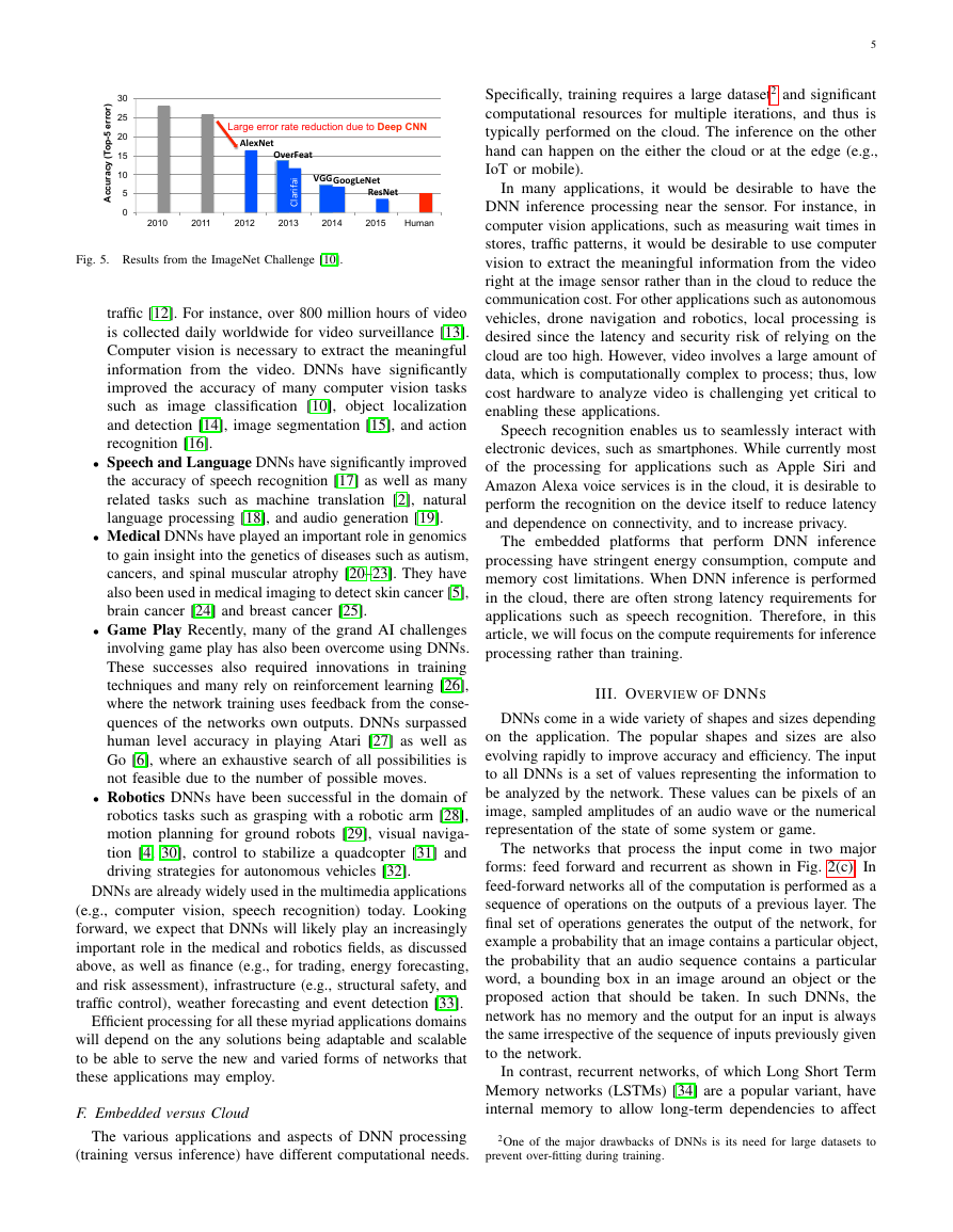
The graph in Fig. 5 shows the performance of the best
entrant in the ImageNet contest over a number of years. One
sees that the accuracy of the algorithms initially had an error
rate of 25% or more. In 2012, a group from the University
of Toronto used graphics processing units (GPUs) for their
high compute capability and a deep neural network approach,
namely AlexNet, and dropped the error rate by approximately
10% [3]. Their accomplishment resulted in an outpouring of
deep learning style algorithms that have resulted in a steady
stream of improvements.
In conjunction with the trend to deep learning approaches
for the ImageNet challenge, there has a been a corresponding
increase in the number of entrants using GPUs. From 2012
when only 4 entrants used GPUs to 2014 when almost all
the entrants (110) were using them. This reflects the almost
complete switch from traditional computer vision approaches
to deep learning-based approaches for the competition.
In 2015, the ImageNet winning entry, ResNet [11], exceeded
human-level accuracy with a top-5 error rate1 below 5%. Since
then, the error rate has dropped below 3% and more focus
is now being placed on more challenging components of the
challenge, such as object detection and localization. These
successes are clearly a contributing factor to the wide range
of applications to which DNNs are being applied.
E. Applications of DNN
Many applications can benefit from DNNs ranging from
multimedia to medical space. In this section, we will provide
examples of areas where DNNs are currently making an impact
and highlight emerging areas where DNNs hope to make an
impact in the future.
• Image and Video Video is arguably the biggest of the
big data. It accounts for over 70% of today’s Internet
1The top-5 error rate is measured based on whether the correct answer
appears in one of the top 5 categories selected by the classifier.
Dog (0.7) Cat (0.1) Bike (0.02) Car (0.02) Plane (0.02) House (0.04) Machine Learning (Inference) Class Probabilities �
5
Specifically, training requires a large dataset2 and significant
computational resources for multiple iterations, and thus is
typically performed on the cloud. The inference on the other
hand can happen on the either the cloud or at the edge (e.g.,
IoT or mobile).
In many applications, it would be desirable to have the
DNN inference processing near the sensor. For instance, in
computer vision applications, such as measuring wait times in
stores, traffic patterns, it would be desirable to use computer
vision to extract the meaningful information from the video
right at the image sensor rather than in the cloud to reduce the
communication cost. For other applications such as autonomous
vehicles, drone navigation and robotics, local processing is
desired since the latency and security risk of relying on the
cloud are too high. However, video involves a large amount of
data, which is computationally complex to process; thus, low
cost hardware to analyze video is challenging yet critical to
enabling these applications.
Speech recognition enables us to seamlessly interact with
electronic devices, such as smartphones. While currently most
of the processing for applications such as Apple Siri and
Amazon Alexa voice services is in the cloud, it is desirable to
perform the recognition on the device itself to reduce latency
and dependence on connectivity, and to increase privacy.
The embedded platforms that perform DNN inference
processing have stringent energy consumption, compute and
memory cost limitations. When DNN inference is performed
in the cloud, there are often strong latency requirements for
applications such as speech recognition. Therefore, in this
article, we will focus on the compute requirements for inference
processing rather than training.
III. OVERVIEW OF DNNS
DNNs come in a wide variety of shapes and sizes depending
on the application. The popular shapes and sizes are also
evolving rapidly to improve accuracy and efficiency. The input
to all DNNs is a set of values representing the information to
be analyzed by the network. These values can be pixels of an
image, sampled amplitudes of an audio wave or the numerical
representation of the state of some system or game.
The networks that process the input come in two major
forms: feed forward and recurrent as shown in Fig. 2(c). In
feed-forward networks all of the computation is performed as a
sequence of operations on the outputs of a previous layer. The
final set of operations generates the output of the network, for
example a probability that an image contains a particular object,
the probability that an audio sequence contains a particular
word, a bounding box in an image around an object or the
proposed action that should be taken. In such DNNs, the
network has no memory and the output for an input is always
the same irrespective of the sequence of inputs previously given
to the network.
In contrast, recurrent networks, of which Long Short Term
Memory networks (LSTMs) [34] are a popular variant, have
internal memory to allow long-term dependencies to affect
Fig. 5. Results from the ImageNet Challenge [10].
traffic [12]. For instance, over 800 million hours of video
is collected daily worldwide for video surveillance [13].
Computer vision is necessary to extract the meaningful
information from the video. DNNs have significantly
improved the accuracy of many computer vision tasks
such as image classification [10], object
localization
and detection [14], image segmentation [15], and action
recognition [16].
• Speech and Language DNNs have significantly improved
the accuracy of speech recognition [17] as well as many
related tasks such as machine translation [2], natural
language processing [18], and audio generation [19].
• Medical DNNs have played an important role in genomics
to gain insight into the genetics of diseases such as autism,
cancers, and spinal muscular atrophy [20–23]. They have
also been used in medical imaging to detect skin cancer [5],
brain cancer [24] and breast cancer [25].
• Game Play Recently, many of the grand AI challenges
involving game play has also been overcome using DNNs.
These successes also required innovations in training
techniques and many rely on reinforcement learning [26],
where the network training uses feedback from the conse-
quences of the networks own outputs. DNNs surpassed
human level accuracy in playing Atari [27] as well as
Go [6], where an exhaustive search of all possibilities is
not feasible due to the number of possible moves.
• Robotics DNNs have been successful in the domain of
robotics tasks such as grasping with a robotic arm [28],
motion planning for ground robots [29], visual naviga-
tion [4, 30], control to stabilize a quadcopter [31] and
driving strategies for autonomous vehicles [32].
DNNs are already widely used in the multimedia applications
(e.g., computer vision, speech recognition) today. Looking
forward, we expect that DNNs will likely play an increasingly
important role in the medical and robotics fields, as discussed
above, as well as finance (e.g., for trading, energy forecasting,
and risk assessment), infrastructure (e.g., structural safety, and
traffic control), weather forecasting and event detection [33].
Efficient processing for all these myriad applications domains
will depend on the any solutions being adaptable and scalable
to be able to serve the new and varied forms of networks that
these applications may employ.
F. Embedded versus Cloud
The various applications and aspects of DNN processing
(training versus inference) have different computational needs.
2One of the major drawbacks of DNNs is its need for large datasets to
prevent over-fitting during training.
0 5 10 15 20 25 30 2010 2011 2012 2013 2014 2015 Human Accuracy (Top-5 error) AlexNet OverFeat GoogLeNet ResNet Clarifai VGG Large error rate reduction due to Deep CNN �
the output. In these networks, some intermediate operations
generate values that are stored internally to the network and
used as inputs to other operations in conjunction with the
processing of a later input. In this article, we will focus on
feed-forward networks as to-date little attention has been given
to hardware acceleration specifically of recurrent networks.
DNNs can be composed of fully-connected (FC, also referred
to as multi-layer perceptrons) as shown in the leftmost layer
of Fig. 2(d). In a fully-connected layer, all output activations
are composed of a weighted sum of all input activations
(i.e., all outputs are connected to all inputs). This requires a
significant amount of storage and computation. Thankfully, in
many applications, we can remove some connections between
the activations by setting the weights to zero without affecting
accuracy. This results in a sparsely-connected layer. A sparsely
connected layer is illustrated in the rightmost layer of Fig. 2(d).
We can also make the computation more efficient by limiting
the number of weights that contribute to an output. This sort of
structured sparsity can arise if each output is only a function
of a fixed-size window of inputs. Even further efficiency can
be gained if the same set of weights are used in the calculation
of every output. This weight sharing can significantly reduce
the storage requirements for weights.
An extremely popular windowed, weight-shared network
arises by structuring the computation as a convolution, as
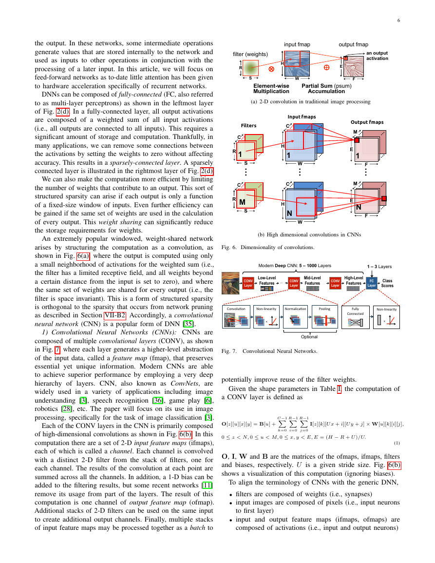
shown in Fig. 6(a), where the output is computed using only
a small neighborhood of activations for the weighted sum (i.e.,
the filter has a limited receptive field, and all weights beyond
a certain distance from the input is set to zero), and where
the same set of weights are shared for every output (i.e., the
filter is space invariant). This is a form of structured sparsity
is orthogonal to the sparsity that occurs from network pruning
as described in Section VII-B2. Accordingly, a convolutional
neural network (CNN) is a popular form of DNN [35].
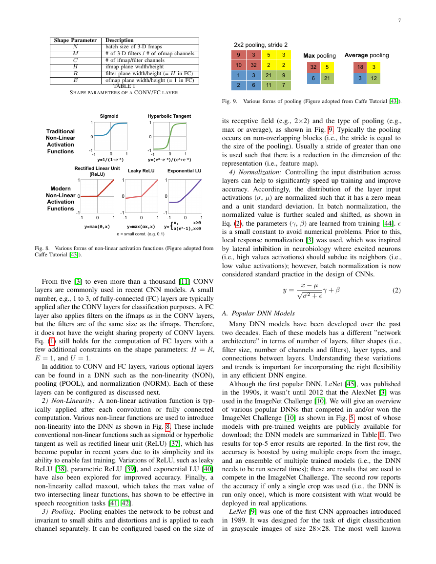
1) Convolutional Neural Networks (CNNs): CNNs are
composed of multiple convolutional layers (CONV), as shown
in Fig. 7, where each layer generates a higher-level abstraction
of the input data, called a feature map (fmap), that preserves
essential yet unique information. Modern CNNs are able
to achieve superior performance by employing a very deep
hierarchy of layers. CNN, also known as ConvNets, are
widely used in a variety of applications including image
understanding [3], speech recognition [36], game play [6],
robotics [28], etc. The paper will focus on its use in image
processing, specifically for the task of image classification [3].
Each of the CONV layers in the CNN is primarily composed
of high-dimensional convolutions as shown in Fig. 6(b). In this
computation there are a set of 2-D input feature maps (ifmaps),
each of which is called a channel. Each channel is convolved
with a distinct 2-D filter from the stack of filters, one for
each channel. The results of the convolution at each point are
summed across all the channels. In addition, a 1-D bias can be
added to the filtering results, but some recent networks [11]
remove its usage from part of the layers. The result of this
computation is one channel of output feature map (ofmap).
Additional stacks of 2-D filters can be used on the same input
to create additional output channels. Finally, multiple stacks
of input feature maps may be processed together as a batch to
6
(a) 2-D convolution in traditional image processing
(b) High dimensional convolutions in CNNs
Fig. 6. Dimensionality of convolutions.
Fig. 7. Convolutional Neural Networks.
potentially improve reuse of the filter weights.
Given the shape parameters in Table I, the computation of
a CONV layer is defined as
C−1
R−1
R−1
O[z][u][x][y] = B[u] +
I[z][k][U x + i][U y + j] × W[u][k][i][j],
0 ≤ z < N, 0 ≤ u < M, 0 ≤ x, y < E, E = (H − R + U )/U.
k=0
i=0
j=0
(1)
O, I, W and B are the matrices of the ofmaps, ifmaps, filters
and biases, respectively. U is a given stride size. Fig. 6(b)
shows a visualization of this computation (ignoring biases).
To align the terminology of CNNs with the generic DNN,
• filters are composed of weights (i.e., synapses)
• input images are composed of pixels (i.e., input neurons
to first layer)
• input and output feature maps (ifmaps, ofmaps) are
composed of activations (i.e., input and output neurons)
R filter (weights) S E F Partial Sum (psum) Accumulation input fmap output fmap Element-wise Multiplication H W an output activation Input fmapsFiltersOutput fmapsRSC…HWC…EFMEFM…RSCHWC1N1M1NModern Deep CNN: 5 – 1000 Layers Class Scores FC Layer CONV Layer Low-Level Features CONV Layer High-Level Features … 1 – 3 Layers Convolu’on Non-linearity × Normaliza’on Pooling Optional Fully Connected × Non-linearity CONV Layer Mid-Level Features �
Shape Parameter
N
M
C
H
R
E
Description
batch size of 3-D fmaps
# of 3-D filters / # of ofmap channels
# of ifmap/filter channels
ifmap plane width/height
filter plane width/height (= H in FC)
ofmap plane width/height (= 1 in FC)
TABLE I
SHAPE PARAMETERS OF A CONV/FC LAYER.
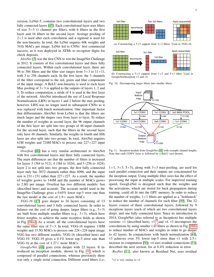
Fig. 8. Various forms of non-linear activation functions (Figure adopted from
Caffe Tutorial [43]).
From five [3] to even more than a thousand [11] CONV
layers are commonly used in recent CNN models. A small
number, e.g., 1 to 3, of fully-connected (FC) layers are typically
applied after the CONV layers for classification purposes. A FC
layer also applies filters on the ifmaps as in the CONV layers,
but the filters are of the same size as the ifmaps. Therefore,
it does not have the weight sharing property of CONV layers.
Eq. (1) still holds for the computation of FC layers with a
few additional constraints on the shape parameters: H = R,
E = 1, and U = 1.
In addition to CONV and FC layers, various optional layers
can be found in a DNN such as the non-linearity (NON),
pooling (POOL), and normalization (NORM). Each of these
layers can be configured as discussed next.
2) Non-Linearity: A non-linear activation function is typ-
ically applied after each convolution or fully connected
computation. Various non-linear functions are used to introduce
non-linearity into the DNN as shown in Fig. 8. These include
conventional non-linear functions such as sigmoid or hyperbolic
tangent as well as rectified linear unit (ReLU) [37], which has
become popular in recent years due to its simplicity and its
ability to enable fast training. Variations of ReLU, such as leaky
ReLU [38], parametric ReLU [39], and exponential LU [40]
have also been explored for improved accuracy. Finally, a
non-linearity called maxout, which takes the max value of
two intersecting linear functions, has shown to be effective in
speech recognition tasks [41, 42].
3) Pooling: Pooling enables the network to be robust and
invariant to small shifts and distortions and is applied to each
channel separately. It can be configured based on the size of
7
Fig. 9. Various forms of pooling (Figure adopted from Caffe Tutorial [43]).
its receptive field (e.g., 2×2) and the type of pooling (e.g.,
max or average), as shown in Fig. 9. Typically the pooling
occurs on non-overlapping blocks (i.e., the stride is equal to
the size of the pooling). Usually a stride of greater than one
is used such that there is a reduction in the dimension of the
representation (i.e., feature map).
4) Normalization: Controlling the input distribution across
layers can help to significantly speed up training and improve
accuracy. Accordingly, the distribution of the layer input
activations (σ, µ) are normalized such that it has a zero mean
and a unit standard deviation. In batch normalization, the
normalized value is further scaled and shifted, as shown in
Eq. (2), the parameters (γ, β) are learned from training [44]. �
is a small constant to avoid numerical problems. Prior to this,
local response normalization [3] was used, which was inspired
by lateral inhibition in neurobiology where excited neurons
(i.e., high values activations) should subdue its neighbors (i.e.,
low value activations); however, batch normalization is now
considered standard practice in the design of CNNs.
y =
γ + β
(2)
x − µ√
σ2 + �
A. Popular DNN Models
Many DNN models have been developed over the past
two decades. Each of these models has a different ”network
architecture” in terms of number of layers, filter shapes (i.e.,
filter size, number of channels and filters), layer types, and
connections between layers. Understanding these variations
and trends is important for incorporating the right flexibility
in any efficient DNN engine.
Although the first popular DNN, LeNet [45], was published
in the 1990s, it wasn’t until 2012 that the AlexNet [3] was
used in the ImageNet Challenge [10]. We will give an overview
of various popular DNNs that competed in and/or won the
ImageNet Challenge [10] as shown in Fig. 5, most of whose
models with pre-trained weights are publicly available for
download; the DNN models are summarized in Table II. Two
results for top-5 error results are reported. In the first row, the
accuracy is boosted by using multiple crops from the image,
and an ensemble of multiple trained models (i.e., the DNN
needs to be run several times); these are results that are used to
compete in the ImageNet Challenge. The second row reports
the accuracy if only a single crop was used (i.e., the DNN is
run only once), which is more consistent with what would be
deployed in real applications.
LeNet [9] was one of the first CNN approaches introduced
in 1989. It was designed for the task of digit classification
in grayscale images of size 28×28. The most well known
Sigmoid 1 -1 0 0 1 -1 y=1/(1+e-x) Hyperbolic Tangent 1 -1 0 0 1 -1 y=(ex-e-x)/(ex+e-x) Rectified Linear Unit (ReLU) 1 -1 0 0 1 -1 y=max(0,x) Leaky ReLU 1 -1 0 0 1 -1 y=max(αx,x) Exponential LU 1 -1 0 0 1 -1 x, α(ex-1), x≥0 x<0 y= α = small const. (e.g. 0.1) Traditional Non-Linear Activation Functions Modern Non-Linear Activation Functions 9 3 5 3 10 32 2 2 1 3 21 9 2 6 11 7 2x2 pooling, stride 2 32 5 6 21 Max pooling Average pooling 18 3 3 12 �
version, LeNet-5, contains two convolutional layers and two
fully connected layers [45]. Each convolutional layer uses filters
of size 5×5 (1 channel per filter), with 6 filters in the first
layer and 16 filters in the second layer. Average pooling of
2×2 is used after each convolution and a sigmoid is used for
the non-linearity. In total, the LeNet requires 60k weights and
341k MACs per image. LeNet led to CNNs’ first commercial
success, as it was deployed in ATMs to recognize digits for
check deposits.
AlexNet [3] was the first CNN to win the ImageNet Challenge
in 2012. It consists of five convolutional layers and three fully
connected layers. Within each convolutional layer, there are
96 to 384 filters and the filter size ranges from 3×3 to 11×11,
with 3 to 256 channels each. In the first layer, the 3 channels
of the filter correspond to the red, green and blue components
of the input image. A ReLU non-linearity is used in each layer.
Max pooling of 3×3 is applied to the outputs of layers 1, 2 and
5. To reduce computation, a stride of 4 is used at the first layer
of the network. AlexNet introduced the use of Local Response
Normalization (LRN) in layers 1 and 2 before the max pooling;
however, LRN was no longer used in subsequent CNNs as it
was replaced with batch normalization. One important factor
that differentiates AlexNet from LeNet is that the filters are
much larger and the shapes vary from layer to layer. To reduce
the number of weights in second layer, the 96 output channels
of the first layer are split into two groups of 48 input channels
for the second layer, such that the filters in the second layer
only have 48 channels. Similarly, the weights in fourth and fifth
layer are also split into two groups. In total, AlexNet requires
61M weights and 724M MACs to process one 227×227 input
image.
Overfeat [46] has a very similar architecture to AlexNet
with five convolutional layers and three fully connected layers.
The main differences are that the number of filters is increased
for layers 3 (384 to 512), 4 (384 to 1024), and 5 (256 to 1024),
layer 2 is not split into two groups, the first fully connected
layer only has 3072 channels rather than 4096, and the input
size is 231×231 rather than 227×227. As a result, the number
of weights grows to 144M and the number of MACs grows
to 2.8G per image. Overfeat has two different models: fast
(described here) and accurate. The accurate model used in the
ImageNet Challenge gives a 0.65% lower top-5 error rate than
the fast model at the cost of 1.9× more MACs
VGG-16 [47] goes deeper to 16 layers consisting of 13
convolutional layers and 3 fully connected layers. In order to
balance out the cost of going deeper, larger filters (e.g., 5×5)
are built from multiple smaller filters (e.g., 3×3), which have
fewer weights, to achieve the same receptive fields as shown
in Fig. 10(a). As a result, all the convolutional layers have
the same filter size of 3×3. In total, VGG-16 requires 138M
weights and 15.5G MACs to process one 224×224 input image.
VGG has two different models: VGG-16 (described here) and
VGG-19. VGG-19 gives a 0.1% lower top-5 error rate than
VGG-16 at the cost of 1.27× more MACs.
GoogLeNet [48] goes even deeper with 22 layers. It in-
troduced an inception module, shown in Fig. 11, which is
composed of parallel connections, whereas previously there
was only a single serial connection. Different sized filters (i.e.,
8
(a) Constructing a 5×5 support from 3×3 filters. Used in VGG-16.
(b) Constructing a 5×5 support from 1×5 and 5×1 filter. Used in
GoogleNet/Inception v3 and v4.
Fig. 10. Decomposing larger filters into smaller filters.
Fig. 11.
Note that each CONV layer is followed by a ReLU (not drawn).
Inception module from GoogleNet [48] with example channel lengths.
1×1, 3×3, 5×5), along with 3×3 max-pooling, are used for
each parallel connection and their outputs are concatenated for
the inception output. Using multiple filter sizes has the effect of
processing the input at multiple scales. For improved training
speed, GoogLeNet is designed such that the weights and
the activations, which are stored for back propagation during
training, could all fit into the GPU memory. In order to reduce
the number of weights, 1×1 filters are applied as a ”bottleneck”
to reduce the number of channels for each filter [49]. The 22
layers consist of three convolutional layers, followed by 9
inceptions layers (each of which are two convolutional layers
deep), and one fully connected layer. Since its introduction in
2014, GoogleNet (also referred to as Inception) has multiple
versions: v1 (described here), v3 3 and v4. v3 decomposes the
convolutions by using smaller 1-D filters as shown in Fig. 10(b)
to reduce number of MACs and weights in order to go deeper
to 42 layers. In conjunctions with batch normalization [44],
v3 achieves over 3% lower top-5 error than v1 with 2.5×
increase in computation [50]. v4 uses residual connections [51],
described the next section, for at 0.4% reduction in error.
ResNet [11], also known as Residual Net, uses residual
3v2 is very similar to v3.
5x5 filter Two 3x3 filters decompose Apply sequentially decompose 5x5 filter 5x1 filter 1x5 filter Apply sequentially 1x1 CONV 3x3 CONV 5x5 CONV 1x1 CONV 1x1 CONV 1x1 CONV 3x3 MAX POOL Input feature map Output feature map C=64 C=192 C=32 C=32 C=128 C=64 C=192 C=64 C=256 �


 2023年江西萍乡中考道德与法治真题及答案.doc
 2012年重庆南川中考生物真题及答案.doc
 2013年江西师范大学地理学综合及文艺理论基础考研真题.doc
 2020年四川甘孜小升初语文真题及答案I卷.doc
 2020年注册岩土工程师专业基础考试真题及答案.doc
 2023-2024学年福建省厦门市九年级上学期数学月考试题及答案.doc
 2021-2022学年辽宁省沈阳市大东区九年级上学期语文期末试题及答案.doc
 2022-2023学年北京东城区初三第一学期物理期末试卷及答案.doc
 2018上半年江西教师资格初中地理学科知识与教学能力真题及答案.doc
 2012年河北国家公务员申论考试真题及答案-省级.doc
 2020-2021学年江苏省扬州市江都区邵樊片九年级上学期数学第一次质量检测试题及答案.doc
 2022下半年黑龙江教师资格证中学综合素质真题及答案.doc