logo资料库

课后习题答案-时间序列分析及应用R语言(第2版).pdf

第1页 / 共304页
第2页 / 共304页
第3页 / 共304页
第4页 / 共304页
第5页 / 共304页
第6页 / 共304页
第7页 / 共304页
第8页 / 共304页
资料共304页,剩余部分请下载后查看
Solutions
Exercise 1.1 Use software to produce the time series plot shown in Exhibit (1.2), page 2. The fol...
Exercise 1.2 Produce the time series plot displayed in Exhibit (1.3), page 3. Use the R code
Exercise 1.3 Simulate a completely random process of length 48 with independent, normal values. R...
Exercise 1.4 Simulate a completely random process of length 48 with independent, chi-square distr...
Exercise 1.5 Simulate a completely random process of length 48 with independent, t-distributed va...
Exercise 1.6 Construct a time series plot with monthly plotting symbols for the Dubuque temperatu...
Exercise 2.1 Suppose E(X) = 2, Var(X) = 9, E(Y) = 0, Var(Y) = 4, and Corr(X,Y) = 0.25. Find:
Exercise 2.2 If X and Y are dependent but Var(X) = Var(Y), find Cov(X + Y, X - Y).
Exercise 2.3 Let X have a distribution with mean m and variance s2 and let Yt = X for all t.
Exercise 2.4 Let {et} be a zero mean white noise processes. Suppose that the observed process is ...
Exercise 2.5 Suppose Yt = 5 + 2t + Xt where {Xt} is a zero mean stationary series with autocovari...
Exercise 2.6 Let {Xt} be a stationary time series and define
Exercise 2.7 Suppose that {Yt} is stationary with autocovariance function gk.
Exercise 2.8 Suppose that {Yt} is stationary with autocovariance function gk. Show that for any f...
Exercise 2.9 Suppose Yt = b0 + b1t + Xt where {Xt} is a zero mean stationary series with autocova...
Exercise 2.10 Let {Xt} be a zero-mean, unit-variance stationary process with autocorrelation func...
Exercise 2.11 Suppose Cov(Xt,Xt-k) = gk is free of t but that E(Xt) = 3t.
Exercise 2.12 Suppose that Yt = et - et-12. Show that {Yt} is stationary and that, for k > 0, i...
Exercise 2.13 Let . For this exercise, assume that the white noise series is normally distributed.
Exercise 2.14 Evaluate the mean and covariance function for each of the following processes. In e...
Exercise 2.15 Suppose that X is a random variable with zero mean. Define a time series by Yt=(-...
Exercise 2.16 Suppose Yt = A + Xt where {Xt} is stationary and A is random but independent of {Xt...
Exercise 2.17 Let {Yt} be stationary with autocovariance function gk. Let . Show that
Exercise 2.18 Let {Yt} be stationary with autocovariance function gk. Define the sample variance as
Exercise 2.19 Let Y1 = q0 + e1 and then for t > 1 define Yt recursively by Yt = q0 + Yt-1 + et....
Exercise 2.20 Consider the standard random walk model where Yt = Yt-1 + et with Y1 = e1.
Exercise 2.21 A random walk with random starting value. Let for t > 0 where Y0 has a distribution...
Exercise 2.22 Let {et} be a zero-mean white noise process and let c be a constant with |c| < 1. D...
Exercise 2.23 Two processes {Zt} and {Yt} are said to be independent if for any time points t1, t...
Exercise 2.24 Let {Xt} be a time series in which we are interested. However, because the measurem...
Exercise 2.25 Suppose where b0, f1, f2,..., fk are constants and A1, A2,..., Ak, B1, B2,..., ...
Exercise 2.26 Define the function . In geostatistics, Gt,s is called the semivariogram.
Exercise 2.27 For a fixed, positive integer r and constant f, consider the time series defined by
Exercise 2.28 (Random cosine wave extended) Suppose that
Exercise 2.29 (Random cosine wave extended more) Suppose that
Exercise 2.30 (Mathematical statistics required) Suppose that
Exercise 3.1 Verify Equation (3.3.2), page 30, for the least squares estimates of b0 and of b1 wh...
Exercise 3.2 Suppose Yt = m + et - et-1. Find . Note any unusual results. In particular, compar...
Exercise 3.3 Suppose Yt = m + et + et-1. Find . Compare your answer to what would have been obtai...
Exercise 3.4 The data file hours contains monthly values of the average hours worked per week in ...
Exercise 3.5 The data file wages contains monthly values of the average hourly wages ($) for work...
Exercise 3.6 The data file beersales contains monthly U.S. beer sales (in millions of barrels) fo...
Exercise 3.7 The data file winnebago contains monthly unit sales of recreational vehicles from Wi...
Exercise 3.8 The data file retail lists total UK (United Kingdom) retail sales (in billions of po...
Exercise 3.9 The data file prescrip gives monthly U.S. prescription costs for the months August 1...
Exercise 3.10 (Continuation of Exercise 3.4) Consider the hours time series again.
Exercise 3.11 (Continuation of Exercise 3.5) Return to the wages series.
Exercise 3.12 (Continuation of Exercise 3.6) Consider the time series in the data file beersales.
Exercise 3.13 (Continuation of Exercise 3.7) Return to the winnebago time series.
Exercise 3.14 (Continuation of Exercise 3.8) The data file retail contains UK monthly retail sale...
Exercise 3.15 (Continuation of Exercise 3.9) Consider again the prescrip time series.
Exercise 3.16 Suppose that a stationary time series, {Yt}, has autocorrelation function of the fo...
Exercise 3.17 Verify Equation (3.2.6), page 29. (Hint: You will need the fact that for -1<f < +1.)
Exercise 3.18 Verify Equation (3.2.7), page 30. (Hint: You will need the two sums
and .)
Exercise 4.1 Use first principles to find the autocorrelation function for the stationary process...
Exercise 4.2 Sketch the autocorrelation functions for the following MA(2) models with parameters ...
Exercise 4.3 Verify that for an MA(1) process
Exercise 4.4 Show that when q is replaced by 1/q, the autocorrelation function for an MA(1) proce...
Exercise 4.5 Calculate and sketch the autocorrelation functions for each of the following AR(1) m...
Exercise 4.6 Suppose that {Yt} is an AR(1) process with -1 < f < +1.
Exercise 4.7 Describe the important characteristics of the autocorrelation function for the follo...
Exercise 4.8 Let {Yt} be an AR(2) process of the special form Yt = f2Yt-2 + et. Use first princip...
Exercise 4.9 Use the recursive formula of Equation (4.3.13), page 72, to calculate and then sketc...
Exercise 4.10 Sketch the autocorrelation functions for each of the following ARMA models:
Exercise 4.11 For the ARMA(1,2) model Yt = 0.8Yt-1 + et + 0.7et-1 + 0.6et-2 show that
Exercise 4.12 Consider two MA(2) processes, one with q1 = q2 = 1/6 and another with q1 = -1 and q...
Exercise 4.13 Let {Yt} be a stationary process with rk= 0 for k > 1. Show that we must have |r1|...
Exercise 4.14 Suppose that {Yt} is a zero mean, stationary process with |r1| < 0.5 and rk= 0 for...
Exercise 4.15 Consider the AR(1) model Yt = fYt-1 + et. Show that if |f|=1 the process cannot...
Exercise 4.16 Consider the “nonstationary” AR(1) model Yt = 3Yt-1 + et.
Exercise 4.17 Consider a process that satisfies the AR(1) equation Yt = ºYt-1 + et.
Exercise 4.18 Consider a process that satisfies the zero-mean, “stationary” AR(1) equation Yt = f...
Exercise 4.19 Consider an MA(6) model with q1 = 0.5, q2 = -0.25, q3 = 0.125, q4 = -0.0625, q5=0...
Exercise 4.20 Consider an MA(7) model with q1 = 1, q2 = -0.5, q3 = 0.25, q4 = -0.125, q5=0.0625...
Exercise 4.21 Consider the model Yt = et-1 - et-2 + 0.5et-3.
Exercise 4.22 Show that the statement “The roots of are greater than 1 in absolute value” is equi...
Exercise 4.23 Suppose that {Yt} is an AR(1) process with r1 = f. Define the sequence {bt} as bt=...
Exercise 4.24 Let {et} be a zero mean, unit variance white noise process. Consider a process that...
Exercise 4.25 Consider an “AR(1)” process satisfying Yt = fYt-1 + et where f can be any number ...
Exercise 5.1 Identify as specific ARIMA models, that is, what are p, d, and q and what are the va...
Exercise 5.2 For each of the ARIMA models below, give the values for E(—Yt) and Var(—Yt).
Exercise 5.3 Suppose that {Yt} is generated according to Yt = et + cet-1+ cet-2+ cet-3++ ce...
Exercise 5.4 Suppose that Yt = A + Bt + Xt where {Xt} is a random walk. First suppose that A and ...
Exercise 5.5 Using the simulated white noise values in Exhibit (5.2), page 88, verify the values ...
Exercise 5.6 Consider a stationary process {Yt}. Show that if r1 < º, —Yt has a larger variance t...
Exercise 5.7 Consider two models:
Exercise 5.8 Consider a nonstationary “AR(1)” process defined as a solution to Equation (5.1.2), ...
Exercise 5.9 Verify Equation (5.1.10), page 90.
Exercise 5.10 Nonstationary ARIMA series can be simulated by first simulating the corresponding s...
Exercise 5.11 The data file winnebago contains monthly unit sales of recreational vehicles (RVs) ...
Exercise 5.12 The data file SP contains quarterly Standard & Poor’s Composite Index of stock pric...
Exercise 5.13 The data file airpass contains international airline passenger monthly totals (in t...
Exercise 5.14 Consider the annual rainfall data for Los Angeles shown in Exhibit (1.1), page 2. T...
Exercise 5.15 Quarterly earnings per share for the Johnson & Johnson company are given in the dat...
Exercise 5.16 The file named gold contains the daily price of gold (in dollars per troy ounce) fo...
Exercise 5.17 Use calculus to show that, for any fixed x > 0, as.
Exercise 6.1 Verify Equation (6.1.3), page 110 for the white noise process.
Exercise 6.2 Verify Equation (6.1.4), page 110 for the AR(1) process.
Exercise 6.3 Verify the line in Exhibit (6.1), page 111, for the values f = ±0.9.
Exercise 6.4 Add new entries to Exhibit (6.1), page 111, for the following values:
Exercise 6.5 Verify Equation (6.1.9), page 111 and Equation (6.1.10) for the MA(1) process.
Exercise 6.6 Verify the line in Exhibit (6.2), page 112, for the values q = ±0.9.
Exercise 6.7 Add new entries to Exhibit (6.2), page 112, for the following values:
Exercise 6.8 Verify Equation (6.1.11), page 112, for the general MA(q) process.
Exercise 6.9 Use Equation (6.2.3), page 113, to verify the value for the lag 2 partial autocorrel...
Exercise 6.10 Show that the general expression for the partial autocorrelation function of an MA(...
We need to show that Equation (6.2.6) satisfies the Yule-walker equations.
Exercise 6.11 Use Equation (6.2.8), page 114, to find the (theoretical) partial autocorrelation f...
Exercise 6.12 From a time series of 100 observations, we calculate r1 = -0.49, r2 = 0.31, r3 = -0...
Exercise 6.13 A stationary time series of length 121 produced sample partial autocorrelation of =...
Exercise 6.14 For a series of length 169, we find that r1 = 0.41, r2 = 0.32, r3 = 0.26, r4 = 0.21...
Exercise 6.15 The sample ACF for a series and its first difference are given in the following tab...
Exercise 6.16 For a series of length 64, the sample partial autocorrelations are given as:
Exercise 6.17 Consider an AR(1) series of length 100 with f = 0.7.
Exercise 6.18 Suppose the {Xt} is a stationary AR(1) process with parameter f but that we can onl...
Exercise 6.19 The time plots of two series are shown below.
Exercise 6.20 Simulate an AR(1) time series with n = 48 and with f = 0.7.
Exercise 6.21 Simulate an MA(1) time series with n = 60 and with q = 0.5.
Exercise 6.22 Simulate an AR(1) time series with n = 48, with
Exercise 6.23 Simulate an AR(1) time series with f = 0.6, with
Exercise 6.24 Simulate an MA(1) time series with q = 0.7, with
Exercise 6.25 Simulate an AR(1) time series of length n = 36 with f = 0.7.
Exercise 6.26 Simulate an MA(1) time series of length n = 48 with q = 0.5.
Exercise 6.27 Simulate an AR(2) time series of length n = 72 with f1 = 0.7 and f2 = -0.4.
Exercise 6.28 Simulate an MA(2) time series of length n = 36 with q1 = 0.7 and q2 = -0.4.
Exercise 6.29 Simulate a mixed ARMA(1,1) model of length n = 60 with f = 0.4 and q = 0.6.
Exercise 6.30 Simulate a mixed ARMA(1,1) model of length n = 100 with f = 0.8 and q = 0.4.
Exercise 6.31 Simulate a nonstationary time series with n = 60 according to the model ARIMA(0,1,1...
Exercise 6.32 Simulate a stationary time series of length n = 36 according to an AR(1) model with...
Exercise 6.33 The data file named deere1 contains 82 consecutive values for the amount of deviati...
Exercise 6.34 The data file named deere2 contains 102 consecutive values for the amount of deviat...
Exercise 6.35 The data file named deere3 contains 57 consecutive measurements recorded from a com...
Exercise 6.36 The data file named robot contains a time series obtained from an industrial robot....
Exercise 6.37 Calculate and interpret the sample EACF for the logarithms of the Los Angeles rainf...
Exercise 6.38 Calculate and interpret the sample EACF for the color property time series. The dat...
Exercise 6.39 The data file named days contains accounting data from the Winegard Co. of Burlingt...
Exercise 7.1 From a series of length 100, we have computed r1 = 0.8, r2 = 0.5, r3 = 0.4, = 2, and...
Exercise 7.2 Assuming that the following data arise from a stationary process, calculate method-o...
Exercise 7.3 If {Yt} satisfies an AR(1) model with f of about 0.7, how long of a series do we nee...
Exercise 7.4 Consider an MA(1) process for which it is known that the process mean is zero. Based...
Exercise 7.5 Given the data Y1 = 10, Y2 = 9, and Y3 = 9.5, we wish to fit an IMA(1,1) model witho...
Exercise 7.6 Consider two different parameterizations of the AR(1) process with nonzero mean:
Exercise 7.7 Verify Equation (7.1.4), page 150.
Exercise 7.8 Consider an ARMA(1,1) model with f = 0.5 and q = 0.45.
Exercise 7.9 Simulate an MA(1) series with q = 0.8 and n = 48.
Exercise 7.10 Simulate an MA(1) series with q = -0.6 and n = 36.
Exercise 7.11 Simulate an MA(1) series with q = -0.6 and n = 48.
Exercise 7.12 Repeat Exercise 7.11 using a sample size of n = 120.
Exercise 7.13 Simulate an AR(1) series with f = 0.8 and n = 48.
Exercise 7.14 Simulate an AR(1) series with f = -0.5 and n = 60.
Exercise 7.15 Simulate an AR(1) series with f = 0.7 and n = 100.
Exercise 7.16 Simulate an AR(2) series with f1 = 0.6, f2 = 0.3, and n = 60.
Exercise 7.17 Simulate an ARMA(1,1) series with f = 0.7, q = 0.4, and n = 72.
Exercise 7.18 Simulate an AR(1) series with f = 0.6, n = 36 but with error terms from a t-distrib...
Exercise 7.19 Simulate an MA(1) series with q = -0.8, n = 60 but with error terms from a t-distri...
Exercise 7.20 Simulate an AR(2) series with f1 = 1.0, f2 = -0.6, n = 48 but with error terms from...
Exercise 7.21 Simulate an ARMA(1,1) series with f = 0.7, q = -0.6, n = 48 but with error terms fr...
Exercise 7.22 Simulate an AR(1) series with f = 0.6, n = 36 but with error terms from a chi-squar...
Exercise 7.23 Simulate an MA(1) series with q = -0.8, n = 60 but with error terms from a chi-squa...
Exercise 7.24 Simulate an AR(2) series with f1 = 1.0, f2 = -0.6, n = 48 but with error terms from...
Exercise 7.25 Simulate an ARMA(1,1) series with f = 0.7, q = -0.6, n = 48 but with error terms fr...
Exercise 7.26 Consider the AR(1) model specified for the color property time series displayed in ...
Exercise 7.27 Exhibit (6.31), page 139, suggested specifying either an AR(1) or possibly an AR(4)...
Exercise 7.28 The data file named deere3 contains 57 consecutive values from a complex machine to...
Exercise 7.29 The data file named robot contains a time series obtained from an industrial robot....
Exercise 7.30 The data file named days contains accounting data from the Winegard Co. of Burlingt...
Exercise 7.31 Simulate a time series of length n = 48 from an AR(1) model with f = 0.7. Use that ...
Exercise 7.32 The industrial color property time series was fitted quite well by an AR(1) model. ...
Exercise 8.1 For an AR(1) model with and n = 100, the lag 1 sample autocorrelation of the residua...
Exercise 8.2 Repeat Exercise 8.1 for an MA(1) model with and n = 100.
Exercise 8.3 Based on a series of length n = 200, we fit an AR(2) model and obtain residual autoc...
Exercise 8.4 Simulate an AR(1) model with n = 30 and f = 0.5.
Exercise 8.5 Simulate an MA(1) model with n = 36 and q = -0.5.
Exercise 8.6 Simulate an AR(2) model with n = 48, f1 = 1.5, and f2 = -0.75.
Exercise 8.7 Fit an AR(3) model by maximum likelihood to the square root of the hare abundance se...
Exercise 8.8 Consider the oil filter sales data shown in Exhibit (1.8), page 7. The data are in t...
Exercise 8.9 The data file named robot contains a time series obtained from an industrial robot. ...
Exercise 8.10 The data file named deere3 contains 57 consecutive values from a complex machine to...
Exercise 8.11 Exhibit (6.31), page 139, suggested specifying either an AR(1) or possibly an AR(4)...
Exercise 9.1 For an AR(1) model with Yt = 12.2, f = -0.5, and m = 10.8,
Exercise 9.2 Suppose that annual sales (in millions of dollars) of the Acme Corporation follow th...
Exercise 9.3 Using the estimated cosine trend on page192:
Exercise 9.4 Using the estimated cosine trend on page192:
Exercise 9.5 Using the seasonal means model without an intercept shown in Exhibit (3.3), page 32:
Exercise 9.6 Using the seasonal means model with an intercept shown in Exhibit (3.4), page 33:
Exercise 9.7 Using the seasonal means model with an intercept shown in Exhibit (3.4), page 33
Exercise 9.8 Consider the monthly electricity generation time series shown in Exhibit (5.8), page...
Exercise 9.9 Simulate an AR(1) process with f = 0.8 and m = 100. Simulate 48 values but set aside...
Exercise 9.10 Simulate an AR(2) process with f1 = 1.5, f2 = -0.75, and m = 100. Simulate 52 value...
Exercise 9.11 Simulate an MA(1) process with q = 0.6 and m = 100. Simulate 36 values but set asid...
Exercise 9.12 Simulate an MA(2) process with q1 = 1, q2 = -0.6, and m = 100. Simulate 36 values b...
Exercise 9.13 Simulate an ARMA(1,1) process with f = 0.7, q = -0.5, and m = 100. Simulate 50 valu...
Exercise 9.14 Simulate an IMA(1,1) process with q = 0.8 and q0 = 0. Simulate 35 values, but set a...
Exercise 9.15 Simulate an IMA(1,1) process with q = 0.8 and q0 = 10. Simulate 35 values, but set ...
Exercise 9.16 Simulate an IMA(2,2) process with q1 = 1, q2 = -0.75, and q0 = 0. Simulate 45 value...
Exercise 9.17 Simulate an IMA(2,2) process with q1 = 1, q2 = -0.75, and q0 = 10. Simulate 45 valu...
Exercise 9.18 Consider the model , where . We assume that b0, b1, and f are known. Show that the ...
Exercise 9.19 Verify Equation (9.3.12), page 196.
Exercise 9.20 Verify Equation (9.3.28), page 199.
Exercise 9.21 The data file named deere3 contains 57 consecutive values from a complex machine to...
Exercise 9.22 The data file named days contains accounting data from the Winegard Co. of Burlingt...
Exercise 9.23 The time series in the data file robot gives the final position in the “x-direction...
Exercise 9.24 Exhibit (9.4), page 206, displayed the forecasts and 95% forecast limits for the sq...
Exercise 9.25 Consider the seasonal means plus linear time trend model for the logarithms of the ...
Exercise 10.1 Based on quarterly data, a seasonal model of the form
Exercise 10.2 An AR model has AR characteristic polynomial
Exercise 10.3 Suppose that {Yt} satisfies
Exercise 10.4 For the seasonal model with |F| < 1, find g0 and rk.
Exercise 10.5 Identify the following as certain multiplicative seasonal ARIMA models:
Exercise 10.6 Verify Equations (10.2.11) on page 232.
Exercise 10.7 Suppose that the process {Yt} develops according to with Yt = et for t = 1, 2, 3, a...
Exercise 10.8 Consider the Alert, Canada, monthly carbon dioxide time series shown in Exhibit (10...
Exercise 10.9 The monthly airline passenger time series, first investigated in Box and Jenkins (1...
Exercise 10.10 Exhibit (5.8), page 99 displayed the monthly electricity generated in the United S...
Exercise 10.11 The quarterly earnings per share for 1960–1980 of the U.S. company Johnson & Johns...
Exercise 10.12 The file named boardings contains monthly data on the number of people who boarded...
chapter11f
chapter12f
chapter13f
chapter14f
chapter15f
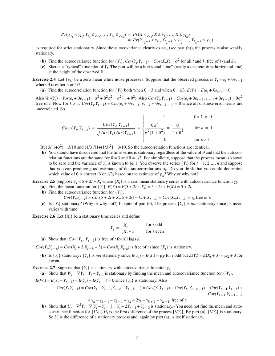
Solutions Manual to Accompany Time Series Analysis with Applications in R, Second Edition by Jonathan D. Cryer and Kung-Sik Chan Solutions by Jonathan Cryer and Xuemiao Hao, updated 7/28/08 CHAPTER 1 Exercise 1.1 Use software to produce the time series plot shown in Exhibit (1.2), page 2. The following R code will produce the graph. > library(TSA); data(larain); win.graph(width=3,height=3,pointsize=8) > plot(y=larain,x=zlag(larain),ylab='Inches',xlab='Previous Year Inches') Exercise 1.2 Produce the time series plot displayed in Exhibit (1.3), page 3. Use the R code > data(color); plot(color,ylab='Color Property',xlab='Batch',type='o') Exercise 1.3 Simulate a completely random process of length 48 with independent, normal values. Repeat this exer- cise several times with a new simulation, that is, a new seed, each time. > plot(ts(rnorm(n=48)),type='o') # If you repeat this command R will use a new “random numbers” each time. If you want to reproduce the same simulation first use the command set.seed(#########) where ######### is an integer of your choice. Exercise 1.4 Simulate a completely random process of length 48 with independent, chi-square distributed values each with 2 degrees of freedom. Use the same R code as in the solution of Exercise 1.3 but replace rnorm(n=48) with rchisq(n=48,df=2). Exercise 1.5 Simulate a completely random process of length 48 with independent, t-distributed values each with 5 degrees of freedom. Construct the time series plot. Use the same R code as in the solution of Exercise 1.3 but replace rnorm(n=48) with rt(n=48,df=5). Exercise 1.6 Construct a time series plot with monthly plotting symbols for the Dubuque temperature series as in Exhibit (1.7), page 6. (Make the plot full screen so that you can see all of detail.) > data(tempdub); plot(tempdub,ylab='Temperature') > points(y=tempdub,x=time(tempdub), pch=as.vector(season(tempdub))) CHAPTER 2 Exercise 2.1 Suppose E(X) = 2, Var(X) = 9, E(Y) = 0, Var(Y) = 4, and Corr(X,Y) = 0.25. Find: (a) Var(X + Y) = Var(X) + Var(Y) +2Cov(X,Y) = 9 + 4 + 2(3*2*0.25) = 16 (b) Cov(X, X + Y) = Cov(X,X) + Cov(X,Y) = 9 + ((3*2*0.25) = 9 + 3/2 = 10.5 (c) Corr(X + Y, X − Y). As in part (a), Var(X−Y) = 10. Then Cov(X + Y, X − Y) = Cov(X,X) − Cov(Y,Y) + Cov(X,Y) − Cov(X,Y) = Var(X) − Var(Y) = 9 − 4 = 5. So ,+( Cov X Y X Y– ) Corr X Y X Y– ,+( ) = ------------------------------------------------------------ ) )Var X Y–( Var X Y+( = 5 ---------------------- 10× 16 = 5 ------------- 4 10 = 0.39528471 Exercise 2.2 If X and Y are dependent but Var(X) = Var(Y), find Cov(X + Y, X − Y). Cov(X + Y, X − Y) = Cov(X,X) − Cov(Y,Y) + Cov(X,Y) − Cov(Y,X) = Var(X) − Var((Y) = 0 Exercise 2.3 Let X have a distribution with mean μ and variance σ2 and let Yt = X for all t. (a) Show that {Yt} is strictly and weakly stationary. Let t1, t2,…, tn be any set of time points and k any time lag. Then 1
( Pr Yt1 < , yt1 Yt2 ≤ … Ytn yt2 , , ≤ ) ytn = = ( ( , < Pr X yt1 < Pr Yt1 k– , ≤ … X ytn X yt2 , yt1 Yt2 ≤ , , ≤ … Ytn yt2 ) , k– k– ≤ ) ytn as required for strict stationarity. Since the autocovariance clearly exists, (see part (b)), the process is also weakly stationary. (b) Find the autocovariance function for {Yt}. Cov(Yt,Yt − k) = Cov(X,X) = σ2 for all t and k, free of t (and k). (c) Sketch a “typical” time plot of Yt. The plot will be a horizontal “line” (really a discrete-time horizontal line) at the height of the observed X. Exercise 2.4 Let {et} be a zero mean white noise processes. Suppose that the observed process is Yt = et + θet − 1 where θ is either 3 or 1/3. (a) Find the autocorrelation function for {Yt} both when θ = 3 and when θ =1/3. E(Yt) = E(et + θet−1) = 0. Also Var(Yt) = Var(et + θet − 1) = σ2 + θ2σ2 = σ2 (1 + θ2). Also Cov(Yt,Yt − 1) = Cov(et + θet − 1, et − 1 + θet − 2) = θσ2 free of t. Now for k > 1, Cov(Yt,Yt − k) = Cov(et + θet − 1, et − k + θet − k − 1) = 0 since all of these error terms are uncorrelated. So Corr Yt Yt ( , ) = k– ( Cov Yt Yt Var Yt --------------------------------------------------- ) k– ) , k– ( )Var Yt ( = 1 for k 0= for k 1= = θ --------------- θ2+ 1 ⎧ ⎪ ⎪ ⎨ ⎪ ⎪ ⎩ θσ2 -------------------------- σ2 1 θ2+( ) 0 1> But 3/(1+32) = 3/10 and (1/3)/[1+(1/3)2] = 3/10. So the autocorrelation functions are identical. (b) You should have discovered that the time series is stationary regardless of the value of θ and that the autocor- relation functions are the same for θ = 3 and θ = 1/3. For simplicity, suppose that the process mean is known to be zero and the variance of Yt is known to be 1. You observe the series {Yt} for t = 1, 2,..., n and suppose that you can produce good estimates of the autocorrelations ρk. Do you think that you could determine which value of θ is correct (3 or 1/3) based on the estimate of ρk? Why or why not? for k Exercise 2.5 Suppose Yt = 5 + 2t + Xt where {Xt} is a zero mean stationary series with autocovariance function γk. (a) Find the mean function for {Yt}. E(Yt) = E(5 + 2t + Xt) = 5 + 2t + E(Xt) = 5 + 2t. (b) Find the autocovariance function for {Yt}. Cov(Yt,Yt − k) = Cov(5 + 2t + Xt, 5 + 2(t − k) + Xt − k) = Cov(Xt,Xt − k) = γk free of t. (c) Is {Yt} stationary? (Why or why not?) In spite of part (b), The process {Yt} is not stationary since its mean varies with time. Exercise 2.6 Let {Xt} be a stationary time series and define (a) Show that Cov Yt Yt ( , Yt = ⎧ ⎨ ⎩ Xt Xt 3+ for t odd for t even ) k– is free of t for all lags k. Cov(Yt,Yt − k) = Cov(Xt + 3,Xt − k + 3) = Cov(Xt,Xt−k) is free of t since {Xt} is stationary. (b) Is {Yt} stationary? {Yt} is not stationary since E(Yt) = E(Xt) = μX for t odd but E(Yt) = E(Xt + 3) = μX + 3 for t even. Exercise 2.7 Suppose that {Yt} is stationary with autocovariance function γk. (a) Show that Wt = ∇Yt = Yt − Yt−1 is stationary by finding the mean and autocovariance function for {Wt}. E(Wt) = E(Yt − Yt − 1) = E(Yt) − E(Yt − 1) = 0 since {Yt} is stationary. Also Cov(Yt,Yt − k) = Cov(Yt − Yt − 1,Yt − k − Yt − k − 1) = Cov(Yt,Yt − k) − Cov(Yt, Yt − k − 1) − Cov(Yt − 1,Yt − k) + Cov(Yt − 1,Yt − k − 1) = γk − γk + 1 − γk − 1 + γk = 2γk − γk + 1 − γk − 1, free of t. (b) Show that Ut = ∇2Yt = ∇[Yt − Yt − 1] = Yt − 2Yt − 1 + Yt − 2 is stationary. (You need not find the mean and auto- covariance function for {Ut}.) Ut is the first difference of the process{∇Yt}. By part (a), {∇Yt} is stationary. So Ut is the difference of a stationary process and, again by part (a), is itself stationary. 2
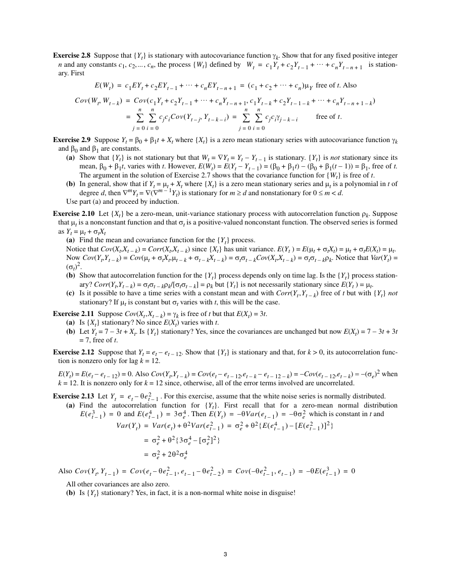
Exercise 2.8 Suppose that {Yt} is stationary with autocovariance function γk. Show that for any fixed positive integer is station- n and any constants c1, c2,..., cn, the process {Wt} defined by ary. First … cnYt c1Yt c2Yt Wt 1+ 1– n– + + + = ( E Wt , Cov Wt Wt ( ) = ) k– c2EYt + + 1– c2Yt + c1EYt = ( Cov c1Yt n ∑= 0= n ∑ 0= i j cjciCov Yt ( + … cnEYt + n– … cnYt ) , j– Yt k– i– + 1– = ( 1+ , n– 1+ n ∑= 0= j c2 + + k– cjciγj + c1 c1Yt n ∑ 0= i + … cn c2Yt 1– )μY + k– k– i– free of t. Also … cnYt free of t. n– + ) 1 k–+ Exercise 2.9 Suppose Yt = β0 + β1t + Xt where {Xt} is a zero mean stationary series with autocovariance function γk and β0 and β1 are constants. (a) Show that {Yt} is not stationary but that Wt = ∇Yt = Yt − Yt − 1 is stationary. {Yt} is not stationary since its mean, β0 + β1t, varies with t. However, E(Wt) = E(Yt − Yt − 1) = (β0 + β1t) − (β0 + β1(t − 1)) = β1, free of t. The argument in the solution of Exercise 2.7 shows that the covariance function for {Wt} is free of t. degree d, then ∇mYt = ∇(∇m − 1Yt) is stationary for m ≥ d and nonstationary for 0 ≤ m < d. (b) In general, show that if Yt = μt + Xt where {Xt} is a zero mean stationary series and μt is a polynomial in t of Use part (a) and proceed by induction. Exercise 2.10 Let {Xt} be a zero-mean, unit-variance stationary process with autocorrelation function ρk. Suppose that μt is a nonconstant function and that σt is a positive-valued nonconstant function. The observed series is formed as Yt = μt + σtXt (a) Find the mean and covariance function for the {Yt} process. Notice that Cov(Xt,Xt − k) = Corr(Xt,Xt − k) since {Xt} has unit variance. E(Yt ) = E(μt + σtXt) = μt + σtE(Xt) = μt. Now Cov(Yt,Yt − k) = Cov(μt + σtXt,μt − k + σt − kXt − k) = σtσt − kCov(Xt,Xt − k) = σtσt − kρk. Notice that Var(Yt) = (σt)2. (b) Show that autocorrelation function for the {Yt} process depends only on time lag. Is the {Yt} process station- ary? Corr(Yt,Yt − k) = σtσt − kρk/[σtσt − k] = ρk but {Yt} is not necessarily stationary since E(Yt ) = μt. Is it possible to have a time series with a constant mean and with Corr(Yt,Yt − k) free of t but with {Yt} not stationary? If μt is constant but σt varies with t, this will be the case. (c) Exercise 2.11 Suppose Cov(Xt,Xt − k) = γk is free of t but that E(Xt) = 3t. (a) Is {Xt} stationary? No since E(Xt) varies with t. (b) Let Yt = 7 − 3t + Xt. Is {Yt} stationary? Yes, since the covariances are unchanged but now E(Xt) = 7 − 3t + 3t = 7, free of t. Exercise 2.12 Suppose that Yt = et − et − 12. Show that {Yt} is stationary and that, for k > 0, its autocorrelation func- tion is nonzero only for lag k = 12. E(Yt) = E(et − et − 12) = 0. Also Cov(Yt,Yt − k) = Cov(et − et − 12,et − k − et − 12 − k) = −Cov(et − 12,et − k) = −(σe)2 when k = 12. It is nonzero only for k = 12 since, otherwise, all of the error terms involved are uncorrelated. Exercise 2.13 Let Yt = 2 et θet 1– – . For this exercise, assume that the white noise series is normally distributed. (a) Find the autocorrelation function for {Yt}. First recall that for a zero-mean normal distribution ( ) ) = 1– 0= = = 3( E et 4( E et ) = θVar et ( – 2 σe { + ) 1– θ2 E et 4( and Var Yt = 1– Var et( 2 σe 2 σe 4 3σe ) ( . Then E Yt θ2Var et 2( ) ) + 1– ]2 θ2 3σe 4 2[ } σe 2θ2σe 4 2 Cov et θet 1– All other covariances are also zero. (b) Is {Yt} stationary? Yes, in fact, it is a non-normal white noise in disguise! 2 Cov θet 1– Cov Yt Yt 2 θet 2– = ) – – et et 1– 1– 1– 1– + + = = = { – – – – ) ( ) ( ) ( , , , Also 2 θσe which is constant in t and 2( [ E et ]2 1– } ) = – 3( θE et 1– ) = 0 3
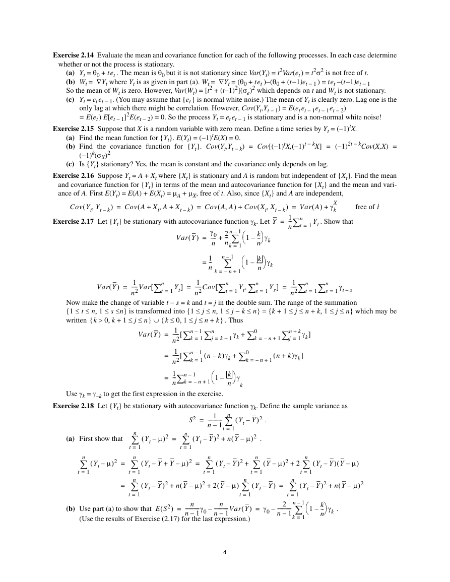
Exercise 2.14 Evaluate the mean and covariance function for each of the following processes. In each case determine whether or not the process is stationary. (a) Yt = θ0 + tet . The mean is θ0 but it is not stationary since Var(Yt) = t2Var(et ) = t2σ2 is not free of t. (b) Wt = ∇Yt where Yt is as given in part (a). Wt = ∇Yt = (θ0 + tet )−(θ0 + (t−1)et − 1 ) = tet −(t−1)et − 1 So the mean of Wt is zero. However, Var(Wt) = [t2 + (t−1)2](σe)2 which depends on t and Wt is not stationary. (c) Yt = et et − 1. (You may assume that {et } is normal white noise.) The mean of Yt is clearly zero. Lag one is the only lag at which there might be correlation. However, Cov(Yt,Yt − 1) = E(et et − 1et − 1et − 2) = E(et ) E[et − 1]2E(et − 2) = 0. So the process Yt = et et − 1 is stationary and is a non-normal white noise! Exercise 2.15 Suppose that X is a random variable with zero mean. Define a time series by Yt = (−1)tX. (a) Find the mean function for {Yt}. E(Yt) = (−1)tE(X) = 0. (b) Find the covariance function for {Yt}. Cov(Yt,Yt − k) = Cov[(−1)tX,(−1)t − kX] = (−1)2t − kCov(X,X) = (−1)k(σX)2 Is {Yt} stationary? Yes, the mean is constant and the covariance only depends on lag. (c) Exercise 2.16 Suppose Yt = A + Xt where {Xt} is stationary and A is random but independent of {Xt}. Find the mean and covariance function for {Yt} in terms of the mean and autocovariance function for {Xt} and the mean and vari- ance of A. First E(Yt) = E(A) + E(Xt) = μA + μX, free of t. Also, since {Xt} and A are independent, , ( ) ( = k– Cov Yt Yt Cov A Xt+ ) Cov Xt Xt + _ Exercise 2.17 Let {Yt} be stationary with autocovariance function γk. Let Y k ⎞ γk ⎛ ---–⎝ 1 ⎠ n _ Var Y Cov A A, +, A Xt γ0 ----- n k– = = ) ( ( ( ) , n 1– 2 ∑+ --- n 1= k k– ) = 1 n∑= --- n t Var A( ) X+ γk free of t· Yt 1= . Show that = 1 --- n k 1– n ∑ n– = 1+ k ⎛ ⎞ γk -----–⎝ 1 ⎠ n _ Var Y ( ) = 1 -----Var n2 n∑[ t ] Yt = 1= 1 -----Cov n2 [ n∑ t Yt n∑, s 1= 1= ] Ys = 1 ----- n2 n∑ n∑t 1= s γt s– 1= Now make the change of variable t − s = k and t = j in the double sum. The range of the summation {1 ≤ t ≤ n, 1 ≤ s ≤n} is transformed into {1 ≤ j ≤ n, 1 ≤ j − k ≤ n} = {k + 1 ≤ j ≤ n + k, 1 ≤ j ≤ n} which may be written +,>{ k ≤ ≤ 0 k } } 1 j n ∪ _ Var Y ( ) j [ = 1= ,≤{ ≤ ≤ 0 1 k+ k j n 1 1–∑ n n∑k ----- n2 1 ----- n2 1 --- n 1–∑= 1–∑ 1= 1+ n– n k n k = [ = k–( n k ⎛ ⎞ γ -----–⎝ 1 ⎠ n k . Thus γk 1+= k 0∑+ k = n– 1+ k+∑ 1= n j γk ] )γk 0∑+ k = n– 1+ k+( n )γk ] Use γk = γ−k to get the first expression in the exercise. Exercise 2.18 Let {Yt} be stationary with autocovariance function γk. Define the sample variance as (a) First show that n ∑ 1= t ( Yt μ– )2 = t = 1 ------------ 1– n _ )2 Yt Y – – _ n∑ ( Yt Y 1= t _ μ–( + n Y )2 )2 . . S2 n∑ ( 1= n ∑ 1= t ( Yt μ– )2 = t _ Y μ–+ )2 = ( – _ Yt Y _ Yt Y – n ∑ 1= n ∑ 1= n ∑ 1= t ( – _ Yt Y _ μ–( 2 Y _ μ–( Y )2 + 2 )2 + t n ∑ 1= _ Yt Y – ( ) = t t ( – n ∑ 1= _ Yt Y _ Yt Y )2 + – _ ) Y μ–( ) _ μ–( n Y )2 ( = n ∑ 1= _ ) ------------Var Y n (Use the results of Exercise (2.17) for the last expression.) n ------------γ0 1– n n 1– E S2( (b) Use part (a) to show that )2 )2 + + = – ) ( ) t t _ μ–( n Y ( n ∑ 1= 1– n ∑ 1= k = γ0 – 2 ------------ 1– n k ⎛ ⎞ γk ---–⎝ 1 ⎠ n . 4
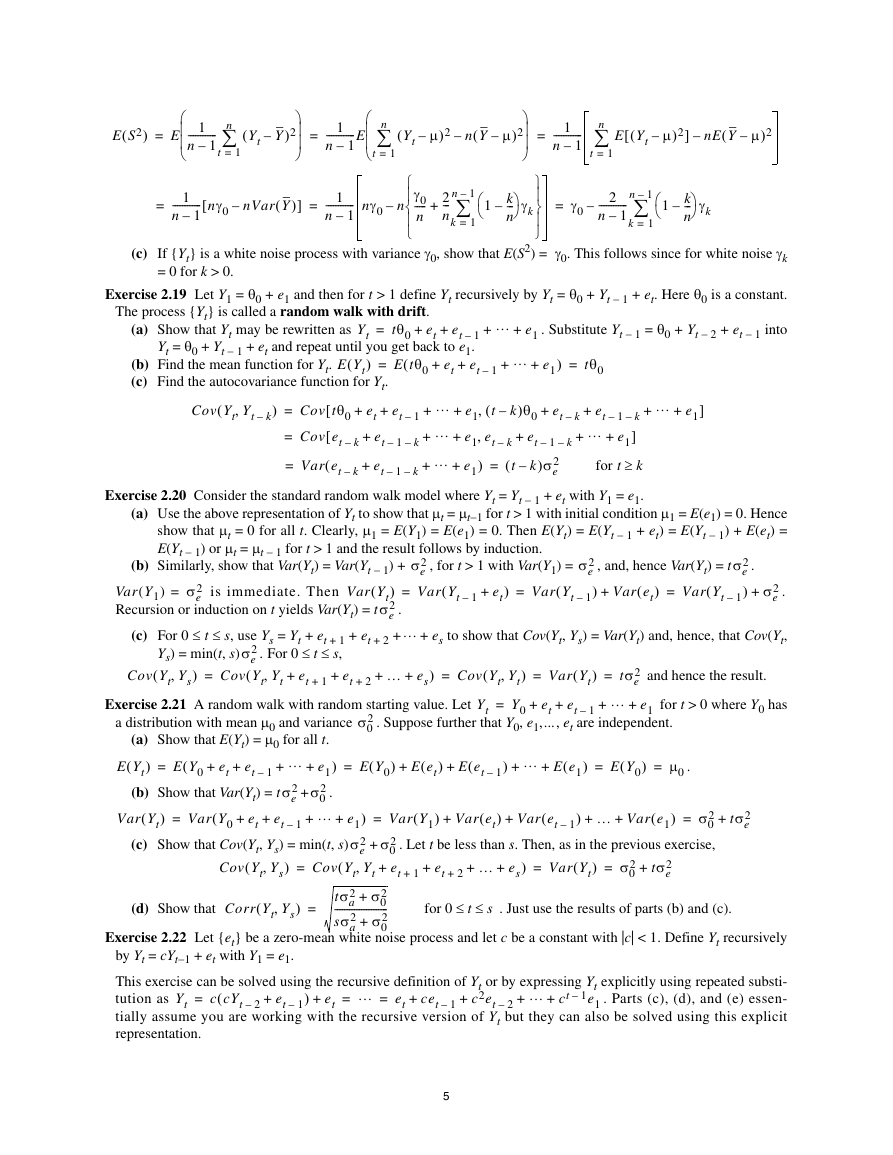
E S2( ) = E ⎛ ⎜ ⎜ ⎝ 1 ------------ 1– n n∑ 1= t _ Yt Y – ( ⎞ ⎟ )2 ⎟ ⎠ = 1 1– ------------E n ⎛ ⎜ ⎜ ⎝ n ∑ 1= t ( Yt μ– )2 – _ μ–( n Y ⎞ ⎟ )2 ⎟ ⎠ = 1 ------------ 1– n n ∑ 1= t [ E Yt μ– ( )2 ] – _ μ–( nE Y )2 = 1 ------------ nγ0 n 1– [ _ nVar Y ( – ) ] = 1 ------------ nγ0 1– n – n γ0 ----- n ⎧ ⎪ ⎨ ⎪ ⎩ n 1– 2 ∑+ --- n 1= k k ⎛ ⎞ γk ---–⎝ 1 ⎠ n ⎫ ⎪ ⎬ ⎪ ⎭ = γ0 – 2 ------------ 1– n n 1– ∑ 1= k k ⎛ ⎞ γk ---–⎝ 1 ⎠ n (c) If {Yt} is a white noise process with variance γ0, show that E(S2) = γ0. This follows since for white noise γk = 0 for k > 0. Exercise 2.19 Let Y1 = θ0 + e1 and then for t > 1 define Yt recursively by Yt = θ0 + Yt − 1 + et. Here θ0 is a constant. + … e1 + . Substitute Yt − 1 = θ0 + Yt − 2 + et − 1 into + … e1 + ) 1– = tθ0 The process {Yt} is called a random walk with drift. + et (a) Show that Yt may be rewritten as 1– Yt = θ0 + Yt − 1 + et and repeat until you get back to e1. + et ( E tθ0 ( E Yt tθ0 Yt et et + = + ) (b) Find the mean function for Yt. = (c) Find the autocovariance function for Yt. + et et + et et Cov tθ0 Cov et Var et Cov Yt Yt [ [ 1– k– k– 1– k– + = = + = ( ( ) , + + + 1– k– k– + … e1 , … e1 , … e1 + + ) + et k–( )θ0 t + et et k– 1– k– 2 k–( )σe = t k– + + et 1– k– … e1 ] + k≥ for t + … e1 + ] Exercise 2.20 Consider the standard random walk model where Yt = Yt − 1 + et with Y1 = e1. (a) Use the above representation of Yt to show that μt = μt−1 for t > 1 with initial condition μ1 = E(e1) = 0. Hence show that μt = 0 for all t. Clearly, μ1 = E(Y1) = E(e1) = 0. Then E(Yt) = E(Yt − 1 + et) = E(Yt − 1) + E(et) = E(Yt − 1) or μt = μt − 1 for t > 1 and the result follows by induction. (b) Similarly, show that Var(Yt) = Var(Yt − 1) + = ( Var(Y1) = Recursion or induction on t yields Var(Yt) = t ) Var Yt 2 σe . (c) For 0 ≤ t ≤ s, use Ys = Yt + et + 1 + et + 2 + is immediate. Then 2 σe Ys) = min(t, s) ( = ) , Cov Yt Ys 2 σe ( . For 0 ≤ t ≤ s, , + + et 1+ Cov Yt Yt et 2+ … es + + ) = 2 σe Var Yt , for t > 1 with Var(Y1) = Var Yt et+ 1– = ( ) ( 2 σe 1– , and, hence Var(Yt) = t ) Var et( + Var Yt = ) ( 2 σe . 2+ ) σe 1– . … + es to show that Cov(Yt, Ys) = Var(Yt) and, hence, that Cov(Yt, , ) ( Cov Yt Yt Y0 Yt = = + ) ( Var Yt + et et 1– 2 tσe = … e1 + + and hence the result. for t > 0 where Y0 has Exercise 2.21 A random walk with random starting value. Let a distribution with mean μ0 and variance 2 σ0 . Suppose further that Y0, e1,..., et are independent. ) ) ( ) ( = = + + = et et E Y0( ( E Y0 Var Yt ) E et( + ) E et + ) … E e1( + (a) Show that E(Yt) = μ0 for all t. … e1 ( + + E Yt 1– 2 2 σ0 σe (b) Show that Var(Yt) = t . + … e1 2 ) σ0 Var Y1( + et 2 2 σ0 σe (c) Show that Cov(Yt, Ys) = min(t, s) . Let t be less than s. Then, as in the previous exercise, + ( , + Cov Yt Yt et 2 σ0 2+ tσa ---------------------- 2 σ0 2+ sσa ) … Var e1( + 2+ … es (d) Show that Corr Yt Ys ) Var et( + ) Var et + Cov Yt Ys Var Y0 Var Yt E Y0( ≤ ≤ 2 tσe for 0 . Just use the results of parts (b) and (c). 2 σ0 μ0 et et 1+ 1– 1– 1– + = = + + + + = = + + + + = = = = s ) ) ( ) ) ( ) ( ( ) ( , ) , t . + 2 tσe Exercise 2.22 Let {et} be a zero-mean white noise process and let c be a constant with |c| < 1. Define Yt recursively by Yt = cYt−1 + et with Y1 = e1. This exercise can be solved using the recursive definition of Yt or by expressing Yt explicitly using repeated substi- tution as . Parts (c), (d), and (e) essen- tially assume you are working with the recursive version of Yt but they can also be solved using this explicit representation. … et … ct ( c cYt 1– e1 c2et et+ cet Yt et 2– 1– 1– 2– + + + + + = = = ) 5
(a) Show that E(Yt) = 0. First E(Y1) = E(e1) = 0. Then E(Yt) = cE(Yt−1) + E(et)= cE(Yt−1) and the result follows by induction on t. (b) Show that Var(Yt) = ( ) = + Var Yt not stationary since Var(Yt) depends on t. Var et cet 1– 2– + ( 2 σe + (1 + c2 +c4 + c2et … … ct + + c2t−2). Is {Yt} stationary? 1– e1 + 2 1 σe ( c2 + + = ) c4 … c2 t + 1–( ) ) = c2t 2 1 – ⎛ ⎞ σe ---------------- ⎝ ⎠ c2– 1 . {Yt} is Alternatively, Var Yt ( ) = = ( Var cYt 1– c3Var Yt ( 2– ( c2Var Yt 2 1 c2+( = ) 2+ ) σe 1– … σe = = 2 1 ( c2Var cYt c2 + + ( 1– c4 … c2 t 1–( 2+ ) σe ) et 2– + + + ) (c) Show that Corr Yt Yt ( , ) = c 1– and, in general, ) et+ = ) σe + ( ) Var Yt 1– --------------------------- ) ( Var Yt Corr Yt Yt ( , ) = ck k– ( ) Var Yt k– -------------------------- ) ( Var Yt for k 0> (Hint: Argue that Yt−1 is independent of et. Then use Cov(Yt, Yt − 1) = Cov(cYt − 1 + et, Yt − 1) Cov Yt Yt ( , ) = 1– So Corr Yt Yt ( , ) = 1– Cov Yt Yt ( , ) = k– Cov cYt ( 1– et+ , Yt So Corr Yt Yt ( , ) = k– ( cVar Yt 1– ) Var Yt 1– --------------------------- ) ( Var Yt ( ) . Next Cov cYt ( Yt ) = 1– --------------------------------------------------- ) 1– = c Var Yt ) = k– , et+ 1– ) ( cVar Yt 1– )Var Yt ( ( cCov cYt 2– c2Cov cYt ) ( k– ( )Var Yt = ( ( = 3– ckVar Yt --------------------------------------------------- ) Var Yt k– ( + = ) ) 2– , et Yt 1– k– , + Yt et ( ) ck Var Yt k– -------------------------- ) ( Var Yt k– , ( c2Cov Yt 2– Yt k– … ckVar Yt ( = = k– ) ) as required. 1– 2 σe -------------- c2– 1 (d) For large t, argue that Var Yt ( ) ≈ 2 σe -------------- c2– 1 and Corr Yt Yt ( , ) ck≈ k– for k 0> so that {Yt} could be called asymptotically stationary. These two results follow from parts (b) and (c). (e) Suppose now that we alter the initial condition and put Y1 = e1 ⁄ ( 1 c2– ) . Show that now {Yt} is station- ary. This part can be solved using repeated substitution to express Yt explicitly as 2– e2 … et … ct ( c cYt c2et et+ cet Yt et 2– 1– 2– + + + + + = = = ) + Then show that Var Yt ( ) = and Corr Yt Yt ( , ) ck= k– for k 0> Exercise 2.23 Two processes {Zt} and {Yt} are said to be independent if for any time points t1, t2,..., tm and s1, }. s2,..., sn, the random variables { Show that if {Zt} and {Yt} are independent stationary processes, then Wt = Zt + Yt is stationary. First, E(Wt) = E(Zt) + E(Yt) = μZ + μY. Then Cov(Wt,Wt − k) = Cov(Zt + Yt, Zt − k + Yt − k) = Cov(Zt,Zt − k) + Cov(Yt,Yt − k) which is free of t since both {Zt} and {Yt} are stationary. } are independent of the random variables { … Ztm … Ysn , Ys1 Ys2 Zt1 Zt2 , , , , , Exercise 2.24 Let {Xt} be a time series in which we are interested. However, because the measurement process itself is not perfect, we actually observe Yt = Xt + et. We assume that {Xt} and {et} are independent processes. We call Xt the signal and et the measurement noise or error process. If {Xt} is stationary with autocorrelation function ρk, show that {Yt} is also stationary with Corr Yt Yt ( , ) = k– for k 1≥ ρk --------------------------- 2 2 σX 1 σe ⁄ + 6 1– ct ------------------e1 1 . c2–
2 2 σe ⁄ σX the signal-to-noise ratio, or SNR. Note that the larger the SNR, the closer the autocorrelation We call function of the observed process {Yt} is to the autocorrelation function of the desired signal {Xt}. First, E(Yt) = E(Xt) + E(et) = μX free of t. Next, for k ≥ 1, Cov(Yt,Yt − k) = Cov(Xt + et, Xt − k + et − k) = Cov(Xt,Xt − k) + Cov(et,et − k) = Cov(Xt,Xt − k) = Var(Xt)ρk which is free of t. Finally, 2 ρk σX -------------------- 2 σe 2+ σX ) ( Cov Yt Yt k– ----------------------------------- ) Var Yt )ρk ( Var Xt --------------------------------- 2+ ) σe Var Xt ρk --------------------------- 2 2 σX 1 σe ⁄ + Corr Yt Yt for k 1≥ , ( k– = = = = ( ( ) , k ∑+ 1= i [ = Yt Ai cos β0 Exercise 2.25 Suppose where β0, f1, f2,..., fk are constants and A1, 2 σi A2,..., Ak, B1, B2,..., Bk are independent random variables with zero means and variances Var(Ai) = Var(Bi) = . Show that {Yt} is stationary and find its covariance function. Compare this exercise with the results for the Random Cosine wave on page 18. First ) ( E Yt ) E Bi + ) Bi + 2πfit 2πfit 2πfit 2πfit ( E Ai cos sin sin β0 β0 = = ( ( ) ] ) ( ( ) ( ) [ ] k ∑+ 1= i Next using the independence of A1, A2,..., Ak, B1, B2,..., Bk and some trig identities we have Cov Yt Ys ( , ) = Cov ⎧ ⎪ ⎨ ⎪ ⎩ k ∑ 1= i [ Ai cos ( 2πfit ) Bi + sin ( 2πfit ) k ∑, ] 1= j [ Aj cos ( 2πfjs ) Bj + sin ( 2πfjs ) ] ⎫ ⎪ ⎬ ⎪ ⎭ = = = k ∑ 1= i k ∑ 1= i k ∑ 1= i k ∑= 1= i Cov Ai { cos ( ( 2πfit ) Ai , cos ( 2πfis ) ) } k ∑+ 1= i Cov Bi { sin ( 2πfjt ) , Bi sin ( 2πfjs ) } { cos ( 2πfit ) cos ( 2πfis ) }Var Ai ( ) k ∑+ 1= i { sin ( 2πfjt ) sin ( 2πfjs ) }Var Bi ( ) { cos ( 2πfi t s–( ) ) + cos ( 2πfi t s+( ) ) } 2 σi ------ 2 k ∑+ 1= i { cos ( 2πfi t s–( ) ) – cos ( 2πfi t s+( ) ) } 2 σi ------ 2 cos ( 2πfi t s–( ) ) 2 σi hence the process is stationary. Exercise 2.26 Define the function 1 [ ( ---E Yt Ys– 2 Γt s, γ0 (a) Show that for a stationary process stationary process has a zero mean. Then Γt s, 2YtYs 1 ---E Yt Ys– 2 1 2 ---E Yt 2 Γt s, )2 = = = = – ( [ ] [ )2 – . In geostatistics, Γt,s is called the semivariogram. ] γ t s– . Without loss of generality, we may assume that the 2+ Ys ] = 1 2[ ---E Yt 2 ] + 1 2[ ---E Ys 2 ] – 1 ---E 2YtYs 2 [ ] = γ0 – γ t s– (b) A process is said to be intrinsically stationary if Γt,s depends only on the time difference |t−s|. Show that the random walk process is intrinsically stationary. + et et 1– ( + es es = For the random walk for t > s we have Yt … e1 + ( … es 1+ 1 2 s–( )σe --- t 2 Exercise 2.27 For a fixed, positive integer r and constant φ, consider the time series defined by … e1 + + … e1 + + + + et Yt Ys– et 1 )2 [ ( = ---E Yt Ys– 2 so that ) ( + = et … es 1– 1 ---Var Yt Ys– 2 1– 1 ( ---Var et 2 et ] = et ) Γt s, = – 1+ 1– 1– + + + + = + = ) ) ( ) and as required. (a) Show that this process is stationary for any value of φ. The mean is clearly zero and Yt = et + φet 1– + φ2et 2– + … φret + . r– 7
Cov Yt Yt ( , ) k– = = + + ( Cov et Cov et φk φk ( + ( 1– + φet + … φket 2+ k– + φ2et 2– φk + … φret + + 1+ et + 1– k– k–( ) 2 r φet k– + , + et r– … φret + r– φ2 2 )σe + 1 k– , et + = ( + 1– + k– φ2et φet k– + 1– k– k–( φ4 … φ2 r + 2– + + … φret + … φret + ) 2φk )σe k– ) r– ) k– r– = 4+ … φk (b) Find the autocorrelation function. We have + φk + + + + = ( ) ( φ2et 2– Var Yt Var et φet 1– Corr Yt Yt ( , ) = k– ( ) 1 = + + … φret )φk ( 1 + --------------------------------------------------------------------------- φ2 φ2 φ4 … φ2r k–( ) + φ4 … φ2r ) r– φ4 … φ2 r + + φ2 1 + + ( + + + + + 2 )σe so that The results in parts (a) and (b) can be simplified for φ ≠ 1 and separately for φ = 1. Exercise 2.28 (Random cosine wave extended) Suppose that Yt = R cos ( 2π f t Φ+( ) ) for t 2 …,±,±,= 0 1 where 0 < f < ½ is a fixed frequency and R and Φ are uncorrelated random variables and with Φ uniformly dis- tributed on the interval (0,1). (a) Show cos )E with a calculation entirely similar to the one on page 18. that E(Yt) = 0 for all 2π f t Φ+( ( 2π f t Φ+( 2π f t Φ+( ( E Yt E R( E R 0= cos cos t. E = = { } { } { } ) ) ( ) ( ) ) ) ) But γk [ E R2 γk (b) Show that the process is stationary with k–( = t and then use the calculations leading up to Equation (2.3.4), page 19 to show that 2πf k cos E R2( 2πf k )E [ 2π f t Φ+( ) cos 1 ---E R2( ) = 2 ) Φ+ = ) Φ+ ) Φ+ k–( t k–( t 2π f ( 2π f ( 2π f ( cos cos cos cos cos E = 2π f t Φ+( ( ) ) ] ( ) ) ) ( ) ] ( ) ) ( ) ( ( [ ) ) cos ( 2π f ( k–( t ) Φ+ ) ) ] Exercise 2.29 (Random cosine wave extended more) Suppose that Yt m ∑= 1= j Rj cos [ 2π fj t Φj+ ( ) ] for t 2 …,±,±,= 0 1 where 0 < f1 < f2 < … < fm < ½ are m fixed frequencies, R1, Φ1, R2, Φ2,…, Rm, Φm are uncorrelated random vari- ables and with each Φj uniformly distributed on the interval (0,1). (a) Show that E(Yt) = 0 for all t. (b) Show that the process is stationary with cos ) ( ) . 2πfj k γk m ∑= 1= 1 --- 2 j 2( E Rj Parts (a) and (b) follow directly from the solution of Exercise (2.28) using the independence. Exercise 2.30 (Mathematical statistics required) Suppose that Yt = R cos [ 2π ft Φ+( ) ] for t 2 …,±,±,= 0 1 where R and Φ are independent random variables and f is a fixed frequency. The phase Φ is assumed to be uni- formly distributed on (0,1), and the amplitude R has a Rayleigh distribution with pdf for r > 0. Show that for each time point t, Yt has a normal distribution. (Hint: Let and X = R . Now find the joint distribution of X and Y. It can also be shown that all of the finite dimensional R distributions are multivariate normal and hence the process is strictly stationary.) re r2 2⁄ = 2π ft Φ+( ) 2π ft Φ+( f r( ) [ cos sin = Y ] [ ) ] – For fixed t and f consider the one-to-one transformation defined by [ sin = Y < ∞– [ 2π ft Φ+( ) cos R X ∞ < < ∞– < , ] X, } Y ∞ R 2π ft Φ+( = . Also X2 + Y2 = R2. Furthermore, ) ] The range for (X,Y) will be { ∂X R∂ ∂Y R∂ ∂X Φ∂ ∂Y Φ∂ = cos sin 2π ft Φ+( ) [ ] ] [ ) 2π ft Φ+( 2πR 2πR sin cos 2π ft Φ+( ) [ ] ] [ ) 2π ft Φ+( and the Jacobian is 2πR– –= 2π X2 Y2+ with inverse Jacobian < 1. Hence the joint density for X and Y is given by 2π X2 Y2+ –( 1 ) ⁄ . The joint density for R and Φ is f r φ,( ) = re r2 2⁄ – for 0 < r and 0 < φ 8
分享到:
收藏