Modern Economy, 2017, 8, 878-887
http://www.scirp.org/journal/me
ISSN Online: 2152-7261
ISSN Print: 2152-7245
The Effects of Negative Nominal Rates on the
Pricing of American Calls: Some Theoretical
and Numerical Insights
Alessia Cafferata1, Pier Giuseppe Giribone2, Marina Resta1
1DIEC, University of Genova, Genova, Italy
2Banca Carige, Genova, Italy
How to cite this paper: Cafferata, A.,
Giribone, P.G. and Resta, M. (2017) The
Effects of Negative Nominal Rates on the
Pricing of American Calls: Some Theoreti-
cal and Numerical Insights. Modern Eco-
nomy, 8, 878-887.
https://doi.org/10.4236/me.2017.87061
Received: May 29, 2017
Accepted: July 10, 2017
Published: July 13, 2017
Copyright © 2017 by authors and
Scientific Research Publishing Inc.
This work is licensed under the Creative
Commons Attribution International
License (CC BY 4.0).
http://creativecommons.org/licenses/by/4.0/
Open Access
Abstract
The article investigates the effects played on options pricing by negative
risk-free rates when the underlying is an equity with null dividends. In such
anomalous conditions, in fact, the fair value at early exercise of the American
Call would not match the value of the European Call with the same financial
features. We originally motivate this assumption with theoretical arguments.
We then move to an empirical investigation where we put at work some
quasi-closed formulas for pricing an American option and the stochastic tri-
nomial trees algorithm. We then draw the conclusion that from a numerical
viewpoint, the bias between the fair value of the American Call and the value
of the corresponding. European Call is mainly due to approximation errors,
which can be mitigated when Trinomial Stochastic Trees are used.
Keywords
American Options, Quasi-Closed Formulas, Negative Interest Rates, Stochastic
Trinomial Trees
1. Introduction
As outlined in a recent note from the Actuarial Association of Europe [1],
nowadays negative nominal interest rates for long term maturities are observable
in both European and American financial markets. In addition to the economic
effects, this led to several technical problems, as the existing pricing models do
not give proper valuations, so that either the financial position cannot be cor-
rectly priced or the results can be questioned [2].
From the financial standpoint, it is therefore necessary to check to what extent
the existing pricing models can be adapted to incorporate negative nominal
DOI: 10.4236/me.2017.87061 July 13, 2017
�
A. Cafferata et al.
rates. This aspect has been already investigated in some research papers: [3] and
[4] discuss the issue for options written on interest rates, both from the practical
and the theoretical viewpoint; [5], focusing on foreign exchange and index op-
tions investigate whether the use of models allowing for negative interest rates
can improve option pricing and implied volatility forecasting; [6], discusses a
new closed form for option pricing that leads to sensitively lower the error in
European options pricing. Besides, [7] adapts the Nelson-Siegel model [8] to in-
clude the negative interest. Finally, the Hull and White model [9], has been re-
cently adapted to calibrate in a more proper way when the underlying is a nega-
tive interest rate [10]; however, to the best of our knowledge, much less efforts
have been devoted to model the effects of negative nominal interest rates in op-
tion pricing for other types of underlying.
In particular, some issues might arise in the case of equity that does not pay
dividends: finding the fair value at early exercise of an American Call might be
tricky, as it could not match the value of a European Call option with the same
parameters. The problem is relevant, because of its corporate implications, as the
option evaluation could make the difference when valuing a firm.
This paper aims to fill in this gap. Our research question is discussing whether
the known approximation formulas can effectively bypass the above highlighted
problems. We illustrate an empirical application, where we compare the estima-
tion of a number of quasi-closed formulas, with that provided by the stochastic
trinomial trees algorithm, and we highlight how the bias between the fair value
of the American Call at early exercise and the value of the corresponding Euro-
pean Call can be strongly mitigated using this latter methodology.
The paper is structured as follows. Section 2 starts by providing a snapshot-
wise demonstration of why the equivalence between the fair value of the Ameri-
can Call at early exercise and the European Call can be violated, for an underly-
ing with null dividends. The section then contains a brief overview about the
approximation schemes employed in the work. Section 3 illustrates the numeri-
cal case study with discussion. Section 4 concludes.
2. Theoretical Issues and Methodology
2.1. On the Violation of the Equivalence between American
and European Call Value
,
C
=
f
(
)
S K T r q σ
,
,
,
,
A
E
E
A
the value of an American Call with
Let us denote by
spot price S , strike price K , time to expiration T , interest rate r , dividend
yield q , and volatility σ. We also denote by
the
corresponding value for a European contingent claim. We focus on the well-
known property [11] according to which in case of an underlying with null divi-
dends we have:
)
S K T r q σ
,
C
=
(
f
,
,
,
,
f
A
(
S K T r
,
,
,
,0,
)
σ
=
f
E
(
S K T r
,
,
,
,0,
)
σ
. (1)
In the case of negative interest rate, (1) might not be satisfied. The value of a
European Call Option, in fact, cannot be lower than the difference between the
879
�
A. Cafferata et al.
spot price and the actual value of the strike price:
)
σ
S T K r
,
,
S T K r
,
,
)
σ
,0,
,0,
≥
(
(
f
f
,
,
A
E
≥
S K
t
−
exp
(
−
rT
)
. (2)
Besides:
f
A
(
S T K r
,
,
,
,0,
)
σ ≥
[
max 0,
S K
t
−
]
, (3)
Joining (2) and (3) we get:
S K S K
t
−
<
−
t
exp
(
−
rT
)
. (4)
(4) clearly holds if
r < , (4) is no more consistent, because the
term in the right-hand side might be either is negative or lower than the value in
the left-hand side, as:
r > . If
1
> .
rT−
exp
0
0
(
)
2.2. Methodology
Pricing American contingent claims has traditionally represented a stimulating
field of analysis as, in contradistinction to European options, they can be exer-
cised at any time before or at maturity. In this case, the Black-Scholes method-
ology cannot be applied, and it is necessary to use approximations schemes. Re-
viewing the related literature requires paramount efforts, besides it is out of the
scope of this work: the interested reader can refer to [11].
Nevertheless, we are mainly concerned with two sub-groups of the above
methods. In the first group, we consider three quasi-closed formulas that con-
veys in different ways the original idea discussed in [12]. In particular, the Bar-
one-Adesi and Whaley-BAW-model [13] is a quadratic approximation method
for pricing exchange-traded American call and put options on commodities and
commodity futures. Using the same notational conventions as in Sec.2.1, we
consider an American Call option whose underlying has a cost of carry equal to
r≥ , ceteris paribus the value of the American Call is equal to
b
that of the European Call so that the Generalized Black-Scholes-GBS-formula for
European contingent claims applies:
= − . When b
r q
=
)
C
(
GBS
E
+
(
A S S
2
*
y
) 2
,
S
<
*
S
; and
AC
= −
S K S
,
≥
*
S
,
is the value of the European Call according to the GBS formula,
A
2
=
*
S
{
1
−
(
N d S
1
*
)
exp
(
−
)
b r T
}
y
2
;
C
A
)GBS
(
EC
where
and:
with:
y
2
Finally,
*
S
(
(
(
+
−
b
2
b
2
2
σ
2
σ
)
1
)
1
− +
= −
*S is the price level such that:
{
1 exp
−
K C S K T r q
,
)
,
σ
−
=
+
S
(
8
r
,
*
,
,
E
2
*
2
σ
)
1 exp
−
(
rT
)
2
.
(
−
(
qT N d S
)
1
*
)
}
y
2
. (5)
The Newton-Raphson algorithm can be then used to solve (5) with initial
value:
880
�
A. Cafferata et al.
S
*
START
=
K
+
∞
*
S
−
K
1 exp
−
(
h
2
)
,
h
2
= −
(
K bT
+
2
σ
T
)
∞
*
S
−
K
,
S
*
∞
=
K
1 2
−
−
(
b
2
2
σ
)
1
− +
(
b
2
2
σ
−
2
)
1
+
8
r
2
σ
1
−
,
1iS + estimator is given by:
)
−
(
K RHS S
=
+
S
i
1
+
i
b S
i
i
(
1
−
b
i
)
,
where:
and:
so that the best
where
RHS S is the right-hand side of (5) at the i-th step.
(
)i
The second method is due to Bjerksund and Stensland—BS1993—and it is more
general than the BAW, as the underlying can be a stock, a future or an exchange
rate, and it is based on a feasible but non-optimal exercise strategy correspond-
ing to a trigger price I [14]. If S > I, it is optimal to exercise the option immedi-
ately, and the value must be equal to the intrinsic value S-K. On the other hand,
if S ≤ I, it will never be optimal to exercise the American call option before expi-
ration, and the value can be found using the Black-Scholes formula. Finally, the
third approximation method is due to Bjerksund and Stensland, again [15]—
BS2002—, and it is based on the extension of the flat boundary concept by di-
viding the time to maturity into two parts, and allowing two separate flat
boundaries in each of them.
An alternative to the above-mentioned approximation methods is represented
by stochastic binomial and trinomial trees. Assuming the stock price to follow a
discrete time process, in the binomial tree scheme [16] the life of the option until
the maturity T is decomposed into N time steps of equal length. At each time
step, the underlying will move either up or down by a specific factor
∆ , with probability p and 1 p− , respec-
u
tively. The value of the America Call exercised at expiration is:
(
N i N i
−
(
tσ
∆ or
tσ
−
Su d
max
(
BIN
E
exp
exp
exp
i N i
−
∑
(
1
rT
i
p
u
p
u
,0
C
K
N i
−
(
)
)
{
)
}
!
=
=
(
−
−
!
−
=
d
)
)
)
)
N
i
=
0
)
(
!
} (
where:
up
{
exp
(
To properly assess
=
t
d
r q
− ∆ −
EC in case of early exercise, at each node of the three the
u d
−
.
)
following pay-off must be applied:
(
,exp
max
K
−
S
i
,
j
{
r t
− ∆
)
p f
u i
,
j
1
+
(
1
+ −
p
u
)
f
i
,
j
}
,
jf
,i
is the value of the Call for the node of position (i,j) in the tree. The
where
initial value of the option can be then derived by way of the standard backward
induction technique. A straightforward extension of this procedure is given by
the trinomial scheme algorithm [17], with the underlying that can now assume
three different states: up, down or unchanged. The increase in the number of
possible states allows to lower the number of necessary steps for the convergence
of the procedure, without any loss in the estimation accuracy. The size of the
881
�
A. Cafferata et al.
(
tσ
2
)
u
=
exp
jumps is usually set to:
2
probability of reaching upward/downward branches is given by:
(
∆ , and
(
σ
exp
exp
exp
exp
exp
b t
∆
σ
−
t
∆
t
∆
)
(
)
=
−
−
=
2
2
2
d
(
{
σ
−
(
tσ
−
∆ , so that the
)
up
{
)
)
(
σ
=
exp
dp
the probability
(
2
−
b t
∆
exp
t
exp
∆
mp of reaching the intermediate node is:
exp
t
∆
−
2
2
)
)
(
−
σ
t
∆
p
m
1
= −
(
σ
)
2
t
∆
}2
−
)
p
u
2
p
d
}2
while
.
3. Examples and Discussion
We consider three scenarios (A, B, and C), and for each of them we compute the
value of the American Call with the approximation schemes illustrated in Sec.
2.2. In detail:
• A represents a typical market situation, with a positive risk-free rate, and
with a dividend-paying stock as underlying;
• B simulates a market situation with a positive risk-free rate, and with a null
dividend stock as underlying: in this case, as
r > , Equation (1) holds;
0
• C considers an atypical situation, with a negative risk-free rate. The underly-
ing stock, likewise in the B case, does not pay any dividend.
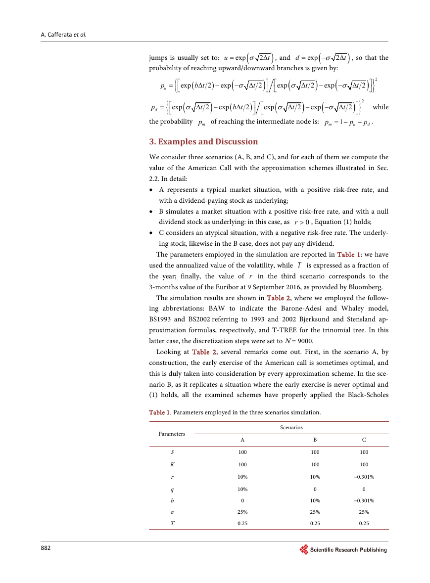
The parameters employed in the simulation are reported in Table 1: we have
used the annualized value of the volatility, while T is expressed as a fraction of
the year; finally, the value of r in the third scenario corresponds to the
3-months value of the Euribor at 9 September 2016, as provided by Bloomberg.
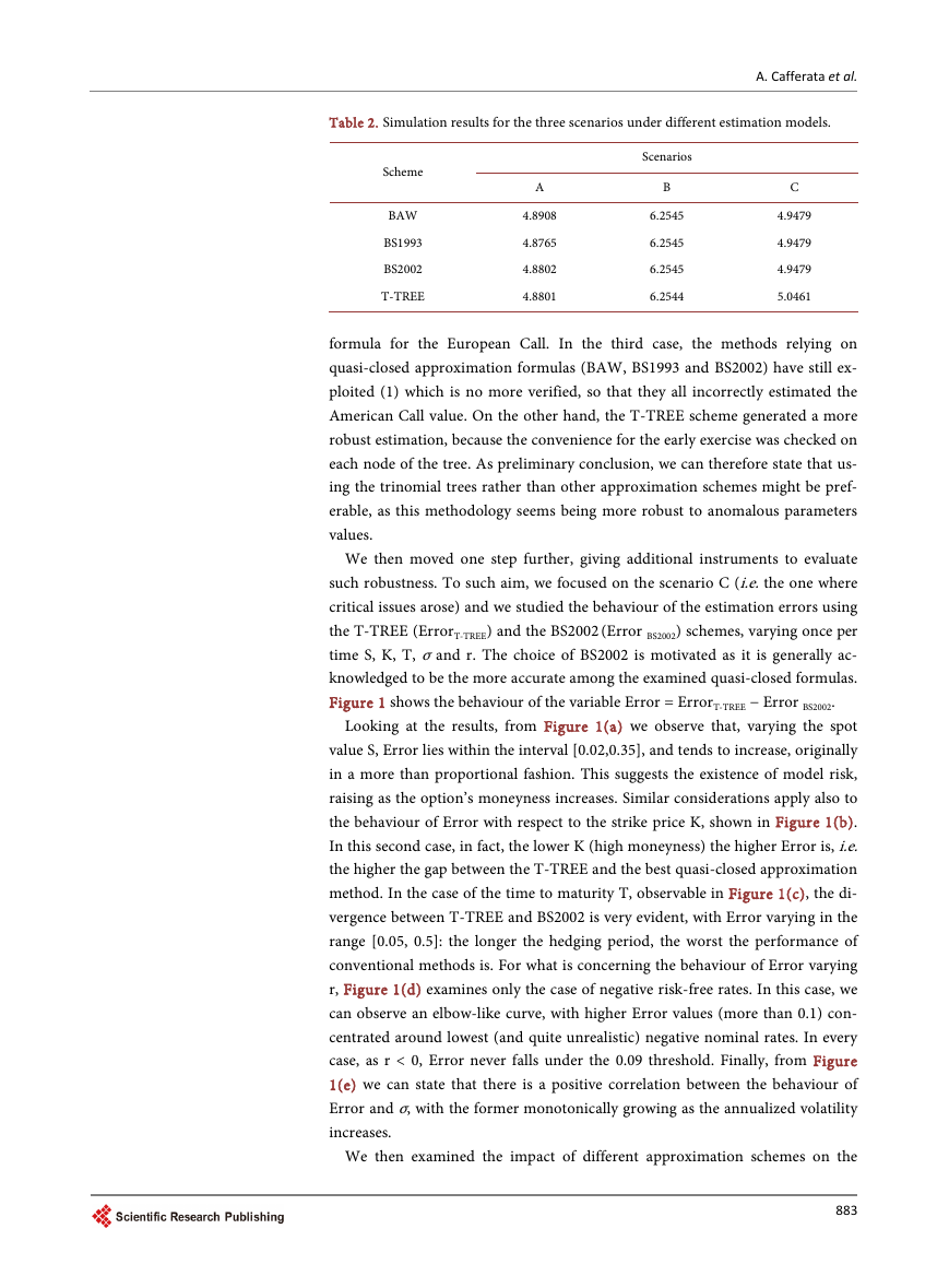
The simulation results are shown in Table 2, where we employed the follow-
ing abbreviations: BAW to indicate the Barone-Adesi and Whaley model,
BS1993 and BS2002 referring to 1993 and 2002 Bjerksund and Stensland ap-
proximation formulas, respectively, and T-TREE for the trinomial tree. In this
latter case, the discretization steps were set to N = 9000.
Looking at Table 2, several remarks come out. First, in the scenario A, by
construction, the early exercise of the American call is sometimes optimal, and
this is duly taken into consideration by every approximation scheme. In the sce-
nario B, as it replicates a situation where the early exercise is never optimal and
(1) holds, all the examined schemes have properly applied the Black-Scholes
Table 1. Parameters employed in the three scenarios simulation.
Parameters
S
K
r
q
b
σ
T
A
100
100
10%
10%
0
25%
0.25
Scenarios
B
100
100
10%
0
10%
25%
0.25
C
100
100
−0.301%
0
−0.301%
25%
0.25
882
�
A. Cafferata et al.
Table 2. Simulation results for the three scenarios under different estimation models.
Scheme
BAW
BS1993
BS2002
T-TREE
A
4.8908
4.8765
4.8802
4.8801
Scenarios
B
6.2545
6.2545
6.2545
6.2544
C
4.9479
4.9479
4.9479
5.0461
formula for the European Call. In the third case, the methods relying on
quasi-closed approximation formulas (BAW, BS1993 and BS2002) have still ex-
ploited (1) which is no more verified, so that they all incorrectly estimated the
American Call value. On the other hand, the T-TREE scheme generated a more
robust estimation, because the convenience for the early exercise was checked on
each node of the tree. As preliminary conclusion, we can therefore state that us-
ing the trinomial trees rather than other approximation schemes might be pref-
erable, as this methodology seems being more robust to anomalous parameters
values.
We then moved one step further, giving additional instruments to evaluate
such robustness. To such aim, we focused on the scenario C (i.e. the one where
critical issues arose) and we studied the behaviour of the estimation errors using
the T-TREE (ErrorT-TREE) and the BS2002 (Error BS2002) schemes, varying once per
time S, K, T, σ and r. The choice of BS2002 is motivated as it is generally ac-
knowledged to be the more accurate among the examined quasi-closed formulas.
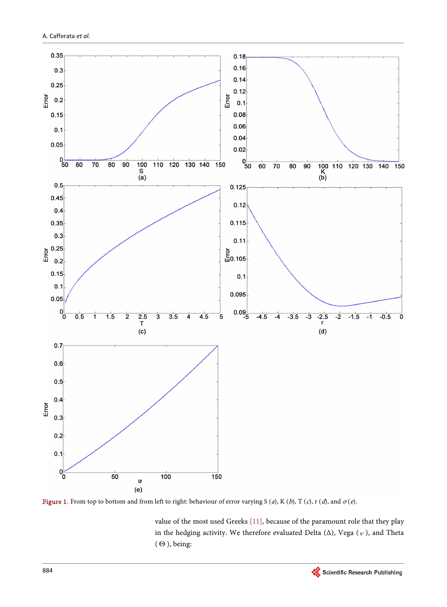
Figure 1 shows the behaviour of the variable Error = ErrorT-TREE − Error BS2002.
Looking at the results, from Figure 1(a) we observe that, varying the spot
value S, Error lies within the interval [0.02,0.35], and tends to increase, originally
in a more than proportional fashion. This suggests the existence of model risk,
raising as the option’s moneyness increases. Similar considerations apply also to
the behaviour of Error with respect to the strike price K, shown in Figure 1(b).
In this second case, in fact, the lower K (high moneyness) the higher Error is, i.e.
the higher the gap between the T-TREE and the best quasi-closed approximation
method. In the case of the time to maturity T, observable in Figure 1(c), the di-
vergence between T-TREE and BS2002 is very evident, with Error varying in the
range [0.05, 0.5]: the longer the hedging period, the worst the performance of
conventional methods is. For what is concerning the behaviour of Error varying
r, Figure 1(d) examines only the case of negative risk-free rates. In this case, we
can observe an elbow-like curve, with higher Error values (more than 0.1) con-
centrated around lowest (and quite unrealistic) negative nominal rates. In every
case, as r < 0, Error never falls under the 0.09 threshold. Finally, from Figure
1(e) we can state that there is a positive correlation between the behaviour of
Error and σ, with the former monotonically growing as the annualized volatility
increases.
We then examined the impact of different approximation schemes on the
883
�
A. Cafferata et al.
Figure 1. From top to bottom and from left to right: behaviour of error varying S (a), K (b), T (c), r (d), and σ (e).
value of the most used Greeks [11], because of the paramount role that they play
in the hedging activity. We therefore evaluated Delta (Δ), Vega (ν), and Theta
( Θ ), being:
884
�
A. Cafferata et al.
C
∆ = ∂
A
S
∂
;
ν
C
= ∂
A
;
σ
∂
C
Θ = ∂
A
∂ ,
T
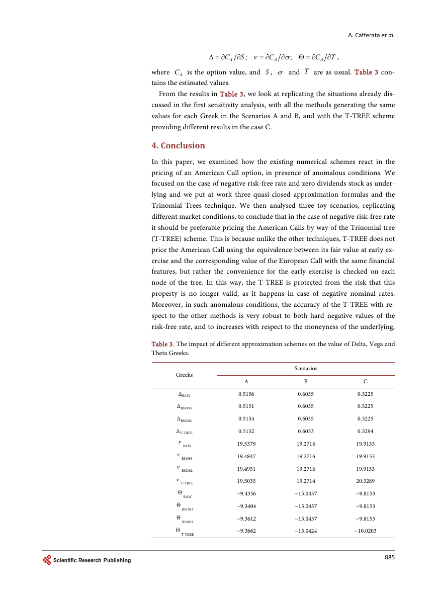
AC is the option value, and S , σ and T are as usual. Table 3 con-
where
tains the estimated values.
From the results in Table 3, we look at replicating the situations already dis-
cussed in the first sensitivity analysis, with all the methods generating the same
values for each Greek in the Scenarios A and B, and with the T-TREE scheme
providing different results in the case C.
4. Conclusion
In this paper, we examined how the existing numerical schemes react in the
pricing of an American Call option, in presence of anomalous conditions. We
focused on the case of negative risk-free rate and zero dividends stock as under-
lying and we put at work three quasi-closed approximation formulas and the
Trinomial Trees technique. We then analysed three toy scenarios, replicating
different market conditions, to conclude that in the case of negative risk-free rate
it should be preferable pricing the American Calls by way of the Trinomial tree
(T-TREE) scheme. This is because unlike the other techniques, T-TREE does not
price the American Call using the equivalence between its fair value at early ex-
ercise and the corresponding value of the European Call with the same financial
features, but rather the convenience for the early exercise is checked on each
node of the tree. In this way, the T-TREE is protected from the risk that this
property is no longer valid, as it happens in case of negative nominal rates.
Moreover, in such anomalous conditions, the accuracy of the T-TREE with re-
spect to the other methods is very robust to both hard negative values of the
risk-free rate, and to increases with respect to the moneyness of the underlying,
Table 3. The impact of different approximation schemes on the value of Delta, Vega and
Theta Greeks.
Greeks
ΔBAW
ΔBS1993
ΔBS2002
ΔT-TREE
ν
BAW
BS1993
BS2002
T-TREE
Θ
ν
ν
ν
BAW
BS1993
BS2002
T-TREE
Θ
Θ
Θ
A
0.5156
0.5151
0.5154
0.5152
19.5379
19.4847
19.4951
19.5035
−9.4356
−9.3404
−9.3612
−9.3662
Scenarios
B
0.6035
0.6035
0.6035
0.6033
19.2716
19.2716
19.2716
19.2714
−15.0457
−15.0457
−15.0457
−15.0424
C
0.5225
0.5225
0.5225
0.5294
19.9153
19.9153
19.9153
20.3289
−9.8153
−9.8153
−9.8153
−10.0203
885
�


 2023年江西萍乡中考道德与法治真题及答案.doc
 2012年重庆南川中考生物真题及答案.doc
 2013年江西师范大学地理学综合及文艺理论基础考研真题.doc
 2020年四川甘孜小升初语文真题及答案I卷.doc
 2020年注册岩土工程师专业基础考试真题及答案.doc
 2023-2024学年福建省厦门市九年级上学期数学月考试题及答案.doc
 2021-2022学年辽宁省沈阳市大东区九年级上学期语文期末试题及答案.doc
 2022-2023学年北京东城区初三第一学期物理期末试卷及答案.doc
 2018上半年江西教师资格初中地理学科知识与教学能力真题及答案.doc
 2012年河北国家公务员申论考试真题及答案-省级.doc
 2020-2021学年江苏省扬州市江都区邵樊片九年级上学期数学第一次质量检测试题及答案.doc
 2022下半年黑龙江教师资格证中学综合素质真题及答案.doc