Introduction to Machine Learning Notes.pdf-资料库

snaildr1234-2186881-4744302542850080157.pdf-第1页.png

第1页 / 共109页

snaildr1234-2186881-4744302542850080157.pdf-第2页.png

第2页 / 共109页

snaildr1234-2186881-4744302542850080157.pdf-第3页.png

第3页 / 共109页

snaildr1234-2186881-4744302542850080157.pdf-第4页.png

第4页 / 共109页

snaildr1234-2186881-4744302542850080157.pdf-第5页.png

第5页 / 共109页

snaildr1234-2186881-4744302542850080157.pdf-第6页.png

第6页 / 共109页

snaildr1234-2186881-4744302542850080157.pdf-第7页.png

第7页 / 共109页

snaildr1234-2186881-4744302542850080157.pdf-第8页.png

第8页 / 共109页

Introduction to Machine Learning 67577 - Fall, 2008 Amnon Shashua School of Computer Science and Engineering The Hebrew University of Jerusalem Jerusalem, Israel 9 0 0 2 r p A 3 2 ] G L . s c [ 1 v 4 6 6 3 . 4 0 9 0 : v i X r a

1 3 4 Contents iii 2 Maximum Likelihood/ Maximum Entropy Duality Bayesian Decision Theory 1.1 Independence Constraints 1.1.1 Example: Coin Toss 1.1.2 Example: Gaussian Density Estimation Incremental Bayes Classiﬁer 1.2 1.3 Bayes Classiﬁer for 2-class Normal Distributions 2.1 ML and Empirical Distribution 2.2 Relative Entropy 2.3 Maximum Entropy and Duality ML/MaxEnt EM Algorithm: ML over Mixture of Distributions 3.1 The EM Algorithm: General 3.2 EM with i.i.d. Data 3.3 Back to the Coins Example 3.4 Gaussian Mixture 3.5 Application Examples page 1 5 7 7 9 10 12 12 14 15 19 21 24 24 26 27 3.5.1 Gaussian Mixture and Clustering 27 3.5.2 Multinomial Mixture and ”bag of words” Application 27 30 Large Margin Classiﬁer as a Quadratic Linear Programming 31 34 36 37 38 39 39 Support Vector Machines and Kernel Functions 4.1 4.2 The Support Vector Machine 4.3 The Kernel Trick 4.3.1 The Homogeneous Polynomial Kernel 4.3.2 The non-homogeneous Polynomial Kernel 4.3.3 The RBF Kernel 4.3.4 Classifying New Instances

iv 5 6 7 8 9 Contents Spectral Analysis I: PCA, LDA, CCA 5.1 PCA: Statistical Perspective 5.1.1 Maximizing the Variance of Output Coordinates 5.1.2 Decorrelation: Diagonalization of the Covariance Matrix 5.2 PCA: Optimal Reconstruction 5.3 The Case n >> m 5.4 Kernel PCA 5.5 Fisher’s LDA: Basic Idea 5.6 Fisher’s LDA: General Derivation 5.7 Fisher’s LDA: 2-class 5.8 5.9 Canonical Correlation Analysis Spectral Analysis II: Clustering 6.1 K-means Algorithm for Clustering LDA versus SVM 6.1.1 Matrix Formulation of K-means 6.2 Min-Cut 6.3 Spectral Clustering: Ratio-Cuts and Normalized-Cuts 6.3.1 Ratio-Cuts 6.3.2 Normalized-Cuts The Formal (PAC) Learning Model 7.1 The Formal Model 7.2 The Rectangle Learning Problem 7.3 Learnability of Finite Concept Classes 7.3.1 The Realizable Case 7.3.2 The Unrealizable Case The VC Dimension 8.1 The VC Dimension 8.2 The Relation between VC dimension and PAC Learning The Double-Sampling Theorem 9.1 A Polynomial Bound on the Sample Size m for PAC Learning 9.2 Optimality of SVM Revisited 10 Appendix Bibliography 41 42 43 46 47 49 49 50 52 54 54 55 58 59 60 62 63 64 65 69 69 73 75 76 77 80 81 85 89 89 95 97 105

1 Bayesian Decision Theory During the next few lectures we will be looking at the inference from training data problem as a random process modeled by the joint probability distribu- tion over input (measurements) and output (say class labels) variables. In general, estimating the underlying distribution is a daunting and unwieldy task, but there are a number of constraints or ”tricks of the trade” so to speak that under certain conditions make this task manageable and fairly eﬀective. To make things simple, we will assume a discrete world, i.e., that the values of our random variables take on a ﬁnite number of values. Consider for example two random variables X taking on k possible values x1, ..., xk and H taking on two values h1, h2. The values of X could stand for a Body Mass Index (BMI) measurement weight/height2 of a person and H stands for the two possibilities h1 standing for the ”person being over-weight” and h2 as the possibility ”person of normal weight”. Given a BMI measurement we would like to estimate the probability of the person being over-weight. The joint probability P (X, H) is a two dimensional array (2-way array) with 2k entries (cells). Each training example (xi, hj) falls into one of those cells, therefore P (X = xi, H = hj) = P (xi, hj) holds the ratio between the number of hits into cell (i, j) and the total number of training examples (assuming the training data arrive i.i.d.). As a result P (hj) = measurement — these are called priors. Likewise, P (xi) = The projections of the array onto its vertical and horizontal axes by sum- ming over columns or over rows is called marginalization and produces i P (xi, hj) the sum over the j’th row is the probability P (H = hj), i.e., the probability of a person being over-weight (or not) before we see any j P (xi, hj) is the probability P (X = xi) which is the probability of receiving such a BMI measurement to begin with — this is often called evidence. Note ij P (xi, hj) = 1. 1

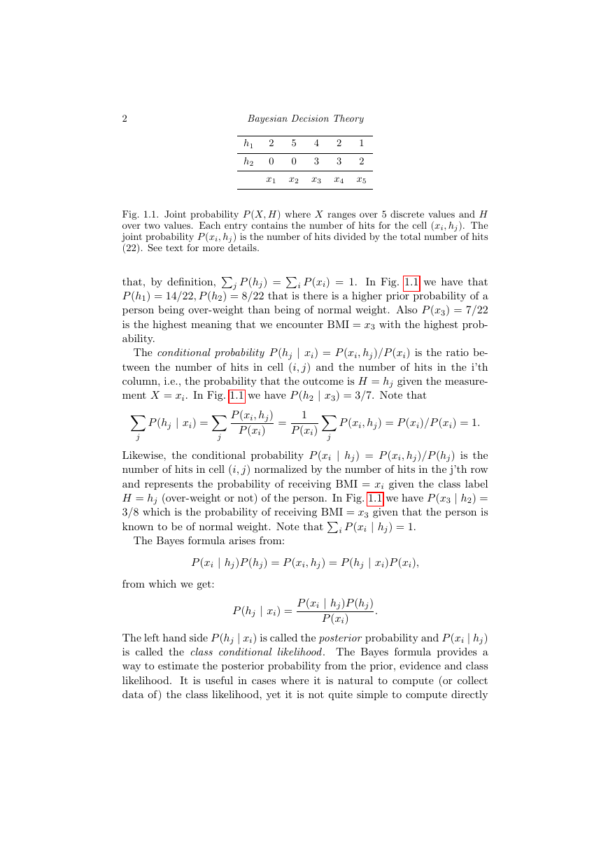
2 Bayesian Decision Theory h1 h2 2 0 5 0 4 3 2 3 1 2 x1 x2 x3 x4 x5 Fig. 1.1. Joint probability P (X, H) where X ranges over 5 discrete values and H over two values. Each entry contains the number of hits for the cell (xi, hj). The joint probability P (xi, hj) is the number of hits divided by the total number of hits (22). See text for more details. that, by deﬁnition, j P (hj) = i P (xi) = 1. In Fig. 1.1 we have that P (h1) = 14/22, P (h2) = 8/22 that is there is a higher prior probability of a person being over-weight than being of normal weight. Also P (x3) = 7/22 is the highest meaning that we encounter BMI = x3 with the highest prob- ability. The conditional probability P (hj | xi) = P (xi, hj)/P (xi) is the ratio be- tween the number of hits in cell (i, j) and the number of hits in the i’th column, i.e., the probability that the outcome is H = hj given the measure- ment X = xi. In Fig. 1.1 we have P (h2 | x3) = 3/7. Note that P (hj | xi) = j j P (xi, hj) P (xi) = 1 P (xi) j P (xi, hj) = P (xi)/P (xi) = 1. Likewise, the conditional probability P (xi | hj) = P (xi, hj)/P (hj) is the number of hits in cell (i, j) normalized by the number of hits in the j’th row and represents the probability of receiving BMI = xi given the class label H = hj (over-weight or not) of the person. In Fig. 1.1 we have P (x3 | h2) = 3/8 which is the probability of receiving BMI = x3 given that the person is known to be of normal weight. Note that i P (xi | hj) = 1. The Bayes formula arises from: P (xi | hj)P (hj) = P (xi, hj) = P (hj | xi)P (xi), from which we get: P (hj | xi) = P (xi | hj)P (hj) . P (xi) The left hand side P (hj | xi) is called the posterior probability and P (xi | hj) is called the class conditional likelihood. The Bayes formula provides a way to estimate the posterior probability from the prior, evidence and class likelihood. It is useful in cases where it is natural to compute (or collect data of) the class likelihood, yet it is not quite simple to compute directly

Bayesian Decision Theory 3 the posterior. For example, given a measurement ”12” we would like to estimate the probability that the measurement came from tossing a pair of dice or from spinning a roulette table. If x = 12 is our measurement, and h1 stands for ”pair of dice” and h2 for ”roulette” then it is natural to compute the class conditional: P (”12” | ”pair of dice”) = 1/36 and P (”12” | ”roulette”) = 1/38. Computing the posterior directly is much more diﬃcult. As another example, consider medical diagnosis. Once it is known that a patient suﬀers from some disease hj, it is natural to evaluate the probabilities P (xi | hj) of the emerging symptoms xi. As a result, in many inference problems it is natural to use the class conditionals as the basic building blocks and use the Bayes formula to invert those to obtain the posteriors. The Bayes rule can often lead to unintuitive results — the one in particu- lar is known as ”base rate fallacy” which shows how an nonuniform prior can inﬂuence the mapping from likelihoods to posteriors. On an intuitive basis, people tend to ignore priors and equate likelihoods to posteriors. The follow- ing example is typical: consider the ”Cancer test kit” problem† which has the following features: given that the subject has Cancer ”C”, the probability of the test kit producing a positive decision ”+” is P (+ | C) = 0.98 (which means that P (− | C) = 0.02) and the probability of the kit producing a neg- ative decision ”-” given that the subject is healthy ”H” is P (− | H) = 0.97 (which means also that P (+ | H) = 0.03). The prior probability of Cancer in the population is P (C) = 0.01. These numbers appear at ﬁrst glance as quite reasonable, i.e, there is a probability of 98% that the test kit will produce the correct indication given that the subject has Cancer. What we are actually interested in is the probability that the subject has Cancer given that the test kit generated a positive decision, i.e., P (C | +). Using Bayes rule: P (C | +) = P (+ | C)P (C) P (+ | C)P (C) = 0.266 P (+) = P (+ | C)P (C) + P (+ | H)P (H) which means that there is a 26.6% chance that the subject has Cancer given that the test kit produced a positive response — by all means a very poor performance. If we draw the posteriors P (h1 |x) and P (h2 | x) using the probability distribution array in Fig. 1.1 we will see that P (h1 |x) > P (h2 | x) for all values of X smaller than a value which is in between x3 and x4. Therefore the decision which will minimize the probability of misclassiﬁcation would † This example is adopted from Yishai Mansour’s class notes on Machine Learning.

4 Bayesian Decision Theory be to choose the class with the maximal posterior: P (hj | x), h∗ = argmax j which is known as the Maximal A Posteriori (MAP) decision principle. Since P (x) is simply a normalization factor, the MAP principle is equivalent to: h∗ = argmax j P (x | hj)P (hj). In the case where information about the prior P (h) is not known or it is known that the prior is uniform, the we obtain the Maximum Likelihood (ML) principle: h∗ = argmax j P (x | hj). The MAP principle is a particular case of a more general principle, known as ”proper Bayes”, where a loss is incorporated into the decision process. Let l(hi, hj) be the loss incurred by deciding on class hi when in fact hj is the correct class. 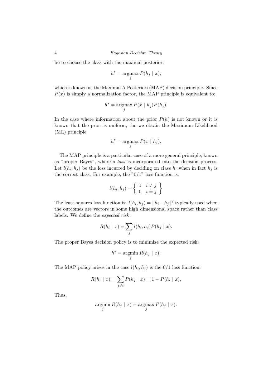For example, the ”0/1” loss function is: 1 i = j 0 i = j l(hi, hj) = The least-squares loss function is: l(hi, hj) = hi − hj2 typically used when the outcomes are vectors in some high dimensional space rather than class labels. We deﬁne the expected risk: R(hi | x) = l(hi, hj)P (hj | x). The proper Bayes decision policy is to minimize the expected risk: j h∗ = argmin j R(hj | x). The MAP policy arises in the case l(hi, hj) is the 0/1 loss function: R(hi | x) = j=i P (hj | x) = 1 − P (hi | x), Thus, argmin j R(hj | x) = argmax j P (hj | x).

资料库

Introduction to Machine Learning Notes.pdf

相关推荐

课程资源

热门标签

最新资料