基于图像分割的立体匹配.pdf

发布时间：2022-05-30 发布人：admin 分类：说明书资料大小：9.36M 资料格式：pdf 举报版权申诉

flxshujie-9704835-4744300845211708303.pdf-第1页.png

第1页 / 共9页

flxshujie-9704835-4744300845211708303.pdf-第2页.png

第2页 / 共9页

flxshujie-9704835-4744300845211708303.pdf-第3页.png

第3页 / 共9页

flxshujie-9704835-4744300845211708303.pdf-第4页.png

第4页 / 共9页

flxshujie-9704835-4744300845211708303.pdf-第5页.png

第5页 / 共9页

flxshujie-9704835-4744300845211708303.pdf-第6页.png

第6页 / 共9页

flxshujie-9704835-4744300845211708303.pdf-第7页.png

第7页 / 共9页

flxshujie-9704835-4744300845211708303.pdf-第8页.png

第8页 / 共9页

文本预览

MeshStereo: A Global Stereo Model with Mesh Alignment Regularization for View Interpolation Chi Zhang2,3∗ Zhiwei Li1 Yanhua Cheng4 Rui Cai1 Hongyang Chao2,3 Yong Rui1 1Microsoft Research 2Sun Yat-Sen University 3SYSU-CMU Shunde International Joint Research Institute, P.R. China 4Institute of Automation, Chinese Academy of Sciences Abstract We present a novel global stereo model designed for view interpolation. Unlike existing stereo models which only out- put a disparity map, our model is able to output a 3D tri- angular mesh, which can be directly used for view inter- polation. To this aim, we partition the input stereo images into 2D triangles with shared vertices. Lifting the 2D trian- gulation to 3D naturally generates a corresponding mesh. A technical difﬁculty is to properly split vertices to multi- ple copies when they appear at depth discontinuous bound- aries. To deal with this problem, we formulate our objec- tive as a two-layer MRF, with the upper layer modeling the splitting properties of the vertices and the lower layer op- timizing a region-based stereo matching. Experiments on the Middlebury and the Herodion datasets demonstrate that our model is able to synthesize visually coherent new view angles with high PSNR, as well as outputting high quality disparity maps which rank at the ﬁrst place on the new chal- lenging high resolution Middlebury 3.0 benchmark. 1. Introduction Stereo model is a key component to generate 3D proxies (either point-clouds [18] or triangular meshes [15]) for view interpolation. Mesh-based approaches are becoming more and more popular [15][16][6][20] because they are faster in rendering speed, have more compact model size and pro- duce better visual effects compared to the point-cloud-based approaches. A typical pipeline to obtain triangular meshes consists of two steps: 1) generate disparity/depth maps by a stereo model, and 2) extract meshes from the estimated disparity maps by heuristic methods, such as triangulating ∗The ﬁrst author was partially supported by the NSF of China under Grant 61173081, the Guangdong Natural Science Foundation, China, un- der Grant S2011020001215, and the Guangzhou Science and Technology Program, China, under Grant 201510010165. Figure 1. A 2D triangulation and a 3D mesh of the Bowling2 test case from Middlebury 2.0 [14] generated by our approach. Blue dots in the left images denote 2D vertices whose splitting proba- bility greater than 0.5. the polyline-simpliﬁed disparity regions [16]. However, due to the separation of the two steps, the ob- tained meshes may not be optimal for the ﬁnal goal of view interpolation. The stereo matching community mainly fo- cuses on producing disparity maps with low pixel-wise er- ror rates [5][9][25][23][17][12][24]. However, pixel-wise accurate disparity maps are not necessary nor sufﬁcient to generate high quality meshes for the task of view interpo- lation. Moreover, the internal structures of a mesh, e.g., alignment of adjacent triangles, which would be helpful for rendering, are not exploited. This observation motivates us to develop an integrated approach for view interpolation, which should have two de- sired properties: 1) the model can naturally produce a mesh structure, such that view interpolation reduces to a simple rendering problem; 2) the model can output a correspond- ing disparity map with high quality to make the rendering results look as natural as possible. In this paper, we propose a stereo model that works on a 2D triangulation of an input view with these two goals in mind. 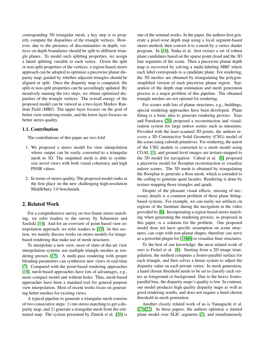In the proposed model, an input image is ﬁrst partitioned into 2D triangular regions according to edge distribution and local visual consistency, as shown in Fig. 1, with com- mon vertices shared by adjacent triangles. To generate the 1

corresponding 3D triangular mesh, a key step is to prop- erly compute the disparities of the triangle vertices. How- ever, due to the presence of discontinuities in depth, ver- tices on depth boundaries should be split to different trian- gle planes. To model such splitting properties, we assign a latent splitting variable to each vertex. Given the split or non-split properties of the vertices, a region-based stereo approach can be adopted to optimize a piecewise planar dis- parity map, guided by whether adjacent triangles should be aligned or split. Once the disparity map is computed, the split or non-split properties can be accordingly updated. By iteratively running the two steps, we obtain optimized dis- parities of the triangle vertices. The overall energy of the proposed model can be viewed as a two-layer Markov Ran- dom Field (MRF). The upper layer focuses on the goal of better view rendering results, and the lower layer focuses on better stereo quality. 1.1. Contribution The contributions of this paper are two-fold 1. We proposed a stereo model for view interpolation whose output can be easily converted to a triangular mesh in 3D. The outputted mesh is able to synthe- size novel views with both visual coherency and high PSNR values. 2. In terms of stereo quality, The proposed model ranks at the ﬁrst place on the new challenging high-resolution Middlebury 3.0 benchmark. 2. Related Work For a comprehensive survey on two-frame stereo match- ing, we refer readers to the survey by Scharstein and Szeliski [14]. And for an overview of point-based view in- terpolation approach, we refer readers to [19]. In this sec- tion, we mainly discuss works on stereo models for image- based rendering that make use of mesh structures. To interpolate a new view, most of state-of-the-art view interpolation systems use multiple triangle meshes as ren- dering proxies [15]. A multi-pass rendering with proper blending parameters can synthesize new views in real-time [7]. Compared with the point-based rendering approaches [18], mesh-based approaches have lots of advantages, e.g., more compact model and without holes. Thus, mesh-based approaches have been a standard tool for general purpose view interpolation. Most of recent works focus on generat- ing better meshes for existing views. A typical pipeline to generate a triangular mesh consists of two consecutive steps: 1) run stereo matching to get a dis- parity map, and 2) generate a triangular mesh from the esti- mated map. The system presented by Zitnick et al. [26] is one of the seminal works. In the paper, the authors ﬁrst gen- erate a pixel-wise depth map using a local segment-based stereo method, then convert it to a mesh by a vertex shader program. In [16], Sinha et al. ﬁrst extract a set of robust plane candidates based on the sparse point cloud and the 3D line segments of the scene. Then a piecewise planar depth map is recovered by solving a multi-labeling MRF where each label corresponds to a candidate plane. For rendering, the 3D meshes are obtained by triangulating the polygon- simpliﬁed version of each piecewise planar region. Sep- aration of the depth map estimation and mesh generation process is a major problem of this pipeline. The obtained triangle meshes are not optimal for rendering. For scenes with lots of planar structures, e.g., buildings, special rendering approaches have been developed. Plane ﬁtting is a basic idea to generate rendering proxies. Xiao and Furukawa [20] proposed a reconstruction and visual- ization system for large indoor scenes such as museums. Provided with the laser-scanned 3D points, the authors re- cover a 3D Constructive Solid Geometry (CSG) model of the scene using cuboids primitives. For rendering, the union of the CSG models is converted to a mesh model using CGAL [1], and ground-level images are texture-mapped to the 3D model for navigation. Cabral et al. [6] proposed a piecewise model for ﬂoorplan reconstruction to visualize indoor scenes. The 3D mesh is obtained by triangulating the ﬂoorplan to generate a ﬂoor mesh, which is extruded to the ceiling to generate quad facades. Rendering is done by texture mapping those triangles and quads. Despite of the pleasant visual effects, missing of nec- essary details is a common problem of these plane ﬁtting- based systems. For example, we can easily see artifacts on regions of the furniture during the navigation in the video provided by [6]. Incorporating a region-based stereo match- ing when generating the rendering proxies, as proposed in this paper, is a solution for the problem. Our proposed model dose not have speciﬁc assumption on scene struc- tures, can cope with non-planar shapes, therefore can serve as a powerful plugin for [16][6] to visualize ﬁner structures. To the best of our knowledge, the most related work of ours is Fickel et al. [8]. Starting from a 2D image trian- gulation, the method computes a fronto-parallel surface for each triangle, and then solves a linear system to adjust the disparity value on each private vertex. In mesh generation, a hand chosen threshold needs to be set to classify each ver- tex as foreground or background. Due to the heavy fronto- parallel bias, the disparity maps’s quality is low. In contrast, our model produces high quality disparity maps as well as good rendering results, and does not require a hand chosen threshold in mesh generation. Another closely related work of us is Yamaguchi et al. [23][22]. In these papers, the authors optimize a slanted plane model over SLIC segments [2], and simultaneously

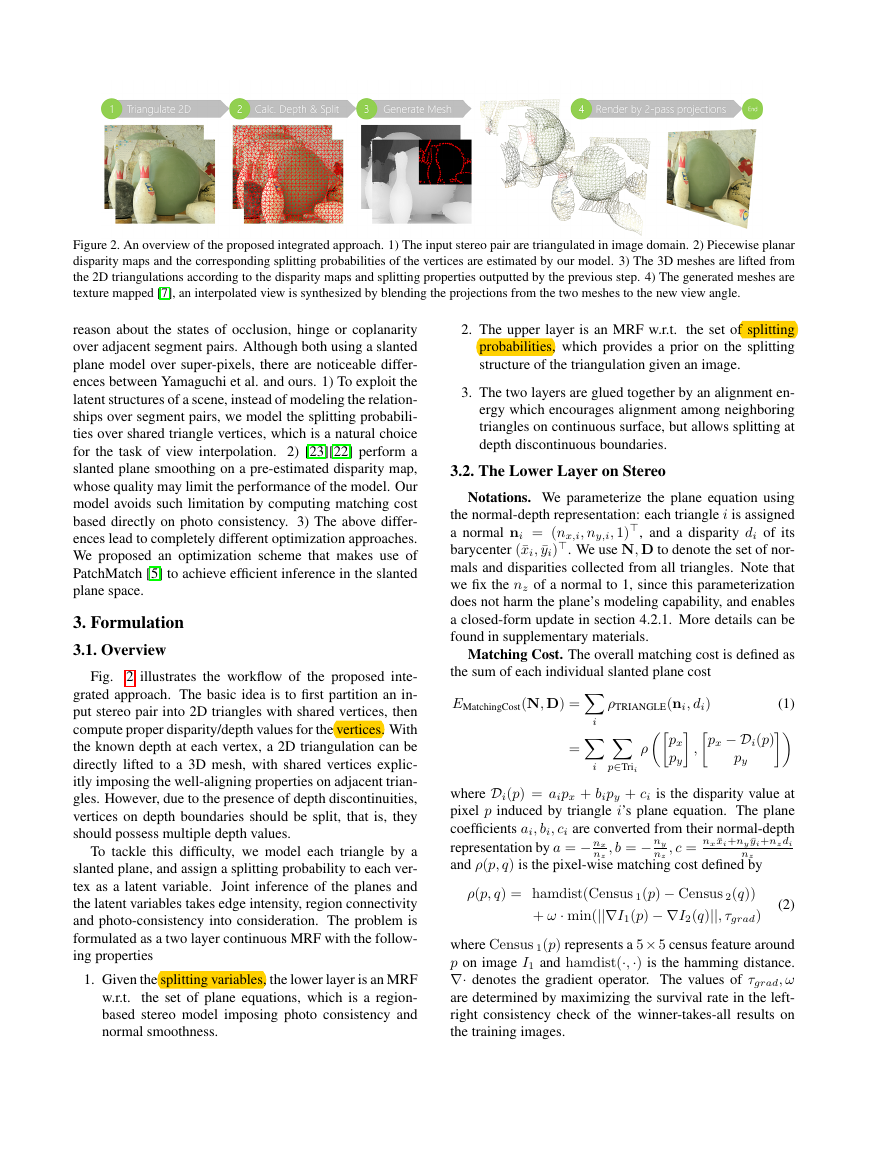
Figure 2. An overview of the proposed integrated approach. 1) The input stereo pair are triangulated in image domain. 2) Piecewise planar disparity maps and the corresponding splitting probabilities of the vertices are estimated by our model. 3) The 3D meshes are lifted from the 2D triangulations according to the disparity maps and splitting properties outputted by the previous step. 4) The generated meshes are texture mapped [7], an interpolated view is synthesized by blending the projections from the two meshes to the new view angle. reason about the states of occlusion, hinge or coplanarity over adjacent segment pairs. Although both using a slanted plane model over super-pixels, there are noticeable differ- ences between Yamaguchi et al. and ours. 1) To exploit the latent structures of a scene, instead of modeling the relation- ships over segment pairs, we model the splitting probabili- ties over shared triangle vertices, which is a natural choice for the task of view interpolation. 2) [23][22] perform a slanted plane smoothing on a pre-estimated disparity map, whose quality may limit the performance of the model. Our model avoids such limitation by computing matching cost based directly on photo consistency. 3) The above differ- ences lead to completely different optimization approaches. We proposed an optimization scheme that makes use of PatchMatch [5] to achieve efﬁcient inference in the slanted plane space. 3. Formulation 3.1. Overview Fig. 2 illustrates the workﬂow of the proposed inte- grated approach. The basic idea is to ﬁrst partition an in- put stereo pair into 2D triangles with shared vertices, then compute proper disparity/depth values for the vertices. With the known depth at each vertex, a 2D triangulation can be directly lifted to a 3D mesh, with shared vertices explic- itly imposing the well-aligning properties on adjacent trian- gles. However, due to the presence of depth discontinuities, vertices on depth boundaries should be split, that is, they should possess multiple depth values. To tackle this difﬁculty, we model each triangle by a slanted plane, and assign a splitting probability to each ver- tex as a latent variable. Joint inference of the planes and the latent variables takes edge intensity, region connectivity and photo-consistency into consideration. The problem is formulated as a two layer continuous MRF with the follow- ing properties 1. Given the splitting variables, the lower layer is an MRF w.r.t. the set of plane equations, which is a region- based stereo model imposing photo consistency and normal smoothness. 2. The upper layer is an MRF w.r.t. the set of splitting probabilities, which provides a prior on the splitting structure of the triangulation given an image. 3. The two layers are glued together by an alignment en- ergy which encourages alignment among neighboring triangles on continuous surface, but allows splitting at depth discontinuous boundaries. 3.2. The Lower Layer on Stereo Notations. We parameterize the plane equation using the normal-depth representation: each triangle i is assigned a normal ni = (nx,i, ny,i, 1), and a disparity di of its barycenter (¯xi, ¯yi). We use N, D to denote the set of nor- mals and disparities collected from all triangles. Note that we ﬁx the nz of a normal to 1, since this parameterization does not harm the plane’s modeling capability, and enables a closed-form update in section 4.2.1. More details can be found in supplementary materials. Matching Cost. The overall matching cost is deﬁned as the sum of each individual slanted plane cost i EMatchingCost(N, D) = = ρTRIANGLE(ni, di) px (1) px − Di(p) ρ , py py p∈Trii i where Di(p) = aipx + bipy + ci is the disparity value at pixel p induced by triangle i’s plane equation. The plane coefﬁcients ai, bi, ci are converted from their normal-depth representation by a = − nx , c = nx ¯xi+ny ¯yi+nzdi and ρ(p, q) is the pixel-wise matching cost deﬁned by ρ(p, q) = hamdist(Census 1(p) − Census 2(q)) + ω · min(||∇I1(p) − ∇I2(q)||, τgrad) , b = − ny (2) nz nz nz where Census 1(p) represents a 5× 5 census feature around p on image I1 and hamdist(·,·) is the hamming distance. ∇· denotes the gradient operator. The values of τgrad, ω are determined by maximizing the survival rate in the left- right consistency check of the winner-takes-all results on the training images.

Normal Smoothness. We impose a smoothness con- straint on the normal pairs of neighboring triangles with similar appearances ENormalSmooth(N) = wij(ni − nj)(ni − nj) (3) i,j∈N where wij = exp(−||ci − cj||1/γ1) measures the similar- ity of the triangles’ mean colors ci, cj, and γ1 controls the inﬂuence of the color difference to the weight. 3.3. The Upper Layer on Splitting Notations. Each shared vertex s is assigned a splitting probability αs. Splitting probabilities of all 2D vertices are denoted by α. Prior on the Splitting Probabilities. We model the prior by a data term and a smoothness term s s,t∈N ESplitPenalty(α) = ESplitSmooth(α) = αs · τs wst(αs − αt)2 (4) (5) where the penalty τs is set adaptively based on the evidence of whether s is located at a strong edge. s, t ∈ N means s and t are neighboring vertices, and wst is a weight deter- mined by the distance of the visual complexity levels of lo- cation s and t. The data term encourages splitting if s is on a strong edge. The smoothness term imposes smoothness if s and t are of similar local visual complexities. Speciﬁcally τs = exp−||∇I 3(xs, ys)||1/γ2 wst = exp(−||k(xs, ys) − k(xt, yt)||/γ3) (6) (7) where {I l, l = 1, 3, 5, 7, 9} is a sequence of progressively gaussian-blurred images using kernel size l × l. k(x, y) is largest scale that pixel (x, y)’s color stay roughly constant {||I l(x, y) − I(x, y)||2 < 10, ∀l ≤ j} (8) k(x, y) = argmax j We discuss how γ2, γ3 are set in the experiment section. 3.4. Gluing the Two Layers So far the two layers have deﬁned two global models for the two sets of variables (i.e., the plane equations and the splitting probabilities), we further combine them together through an alignment term. The new term demands a strong alignment on shared vertices located at continuous surfaces, while allows a shared vertex to posses multiple depth values if its splitting probability is high wij ·Di(xs, ys) − Dj(xs, ys)2 (1 − αs) s (9) EAlignment(N, D, α) = · i,j∈Gs 1 2 Algorithm 1 Optimize EALL RandomInit(N, D); α = 1; repeat M-step: ﬁx α, minimize ELOWER with respect to N, D by Algorithm 2. E-step: ﬁx N, D, minimize EUPPER with respect to α by solving (13) using Cholesky decomposition. until converged where Gs denotes the set of triangles sharing the vertex s, and recall that Di(xs, ys) deﬁned in (1) denotes disparity of s evaluated by triangle i’s plane equation. Therefore, at regions with continuous depth (αs close to zero), the align- ment term will encourage triangles to have their disparities agreed on s. At depth discontinuous boundaries (αs close to 1), it allows the triangles in Gs to stick to their own dis- parities with little penalty. Note that ENormalSmooth and EAlignment together impose a complete second-order smoothness on the disparity ﬁeld. That is, the energy terms do not penalize slanted disparity planes. 3.5. Overall Energy Combining the two layers and the alignment energy, we obtain the overall objective function EALL(N, D, α) = EMatchingCost + λNS · ENormalSmooth (10) + λAL · EAlignment + λSP · ESplitPenalty + λSS · ESplitSmooth where λ× are scaling factors. For the ease of presentation in the next section, we introduce the following notations EUPPER = λSPESplitPenalty + λSSESplitSmooth + λALEAlignment (11) ELOWER = EMatchingCost + λNSENormalSmooth + λALEAlignment (12) 4. Optimization The overall energy EALL in (10) poses a challenging op- timization problem since the variables are all continuous and tightly coupled. We propose an EM-like approach to optimize the energy, in which the splitting probabilities α are treated as latent variables, and the plane equations N, D are treated as model parameters. Optimization proceeds by iteratively updating α (E-step), which can be solved in closed-form, and N, D (M-step), which is optimized by a region-based stereo model through quadratic relaxation. The method is summarized in Algorithm 1. 4.1. E-Step: Optimize EUPPER By ﬁxing N, D, Optimizing EALL is equivalent to opti- mize EUPPER, which is listed as follow with some algebraic

s s α min s,t∈N cAL(s) rearrangement wst(αs−αt)2+ τs−cAL(s)αs+ where cAL(s) = is the current alignment cost at vertex s. And 2 wij·Di(xs, ys)−Dj(xs, ys)2 s cAL(s) is now a constant independent of α. Since (13) is quadratic in α, we can update α in closed-form by solving the positive semi-deﬁnite linear system obtained by setting the deriva- tives of (13) to zeros. We solve the linear system using Cholesky decomposition. 4.2. M-step: Optimize ELOWER i,j∈Gs (13) 1 By ﬁxing α, Optimizing EALL is equivalent to optimize ELOWER min N,D EMatchingCost(N, D) + λNSENormalSmooth(N, D) + λALEAlignment(N, D) (14) (15) However, this subproblem is not yet directly solvable due to the non-convexity of ρ(ni, di). Inspired by [25][21], we adopt the quadratic splitting technique to relax the energy ERELAXED(N, D,N,D) EMatchingCost(N,D) + min N,D,N,D ≡ min N,D,N,D θ 2 + λNSENormalSmooth(N, D) + λALEAlignment(N, D) ECouple(N, D,N,D) (Πi−Πi)Σ(Πi−Πi) (16) ECouple(N, D,N,D) = trols the coupling strength between Πi and Πi. As the θ in i , di], and Σ = diag(σn, σn, σn, σd) con- where Πi = [n in which (15) goes to inﬁnity, minimizing ERELAXED is equivalent to minimizing ELOWER. We found that increasing θ from 0 to 100 in ten levels using the smooth step function offers good numerical stability. The values of σd, σn are set to the in- verse variances of the disparities and normals respectively from the training images. i 4.2.1 Optimize ERELAXED We propose an algorithm similar to that in [25] to optimize the relaxed energy. The algorithm operates by alternatively updating N,D and N, D, which is summarized in Algo- Update N,D. By ﬁxing N, D, Problem (15) reduces to ECouple(N, D,N,D) minN,D EMatchingCost(N,D) + rithm 2. θ 2 (17) Algorithm 2 Optimize ELOWER set θ to zero repeat repeat Minimize (17) by PatchMatch [4][5]. Minimize (18) by Cholesky decomposition. until converged Increase θ until converged This is a Nearest Neighbor Field (NNF) searching problem in disparity plane space, which can be efﬁciently optimized by PatchMatch [5][4]. Update N, D. By ﬁxing N,D, problem (15) reduces to θ ECouple(N, D,N,D) + λNSENormalSmooth(N, D) + λALEAlignment(N, D) min N,D (18) 2 It is easy to verify that all the three terms in (18) are quadratic in N, D (details in supplementary materi- als). Therefore the update can be done in closed-form by Cholesky decomposition. Note that different from [25], we are working on triangles instead of image pixels. Therefore the update is much faster and scales to large size images. 5. Rendering 5.1. Triangulation and Mesh Generation We propose a simple but effective method for image do- main triangulation. First we partition the input image into SLIC [2] segments and perform a joint polyline simpliﬁ- cation on each segment boundary. Second the output is obtained by delaunay triangulating each polygonized SLIC segment. We also try other triangulation approach, such as the one presented in Fickel et al. [8]. We refer interested readers to [8] for details. Given the estimated piecewise planar disparity map and the splitting variables, a 3D mesh is lifted from the triangu- lation, where vertices with splitting probabilities > 0.5 are split to multiple instances, or merged to their median value otherwise. 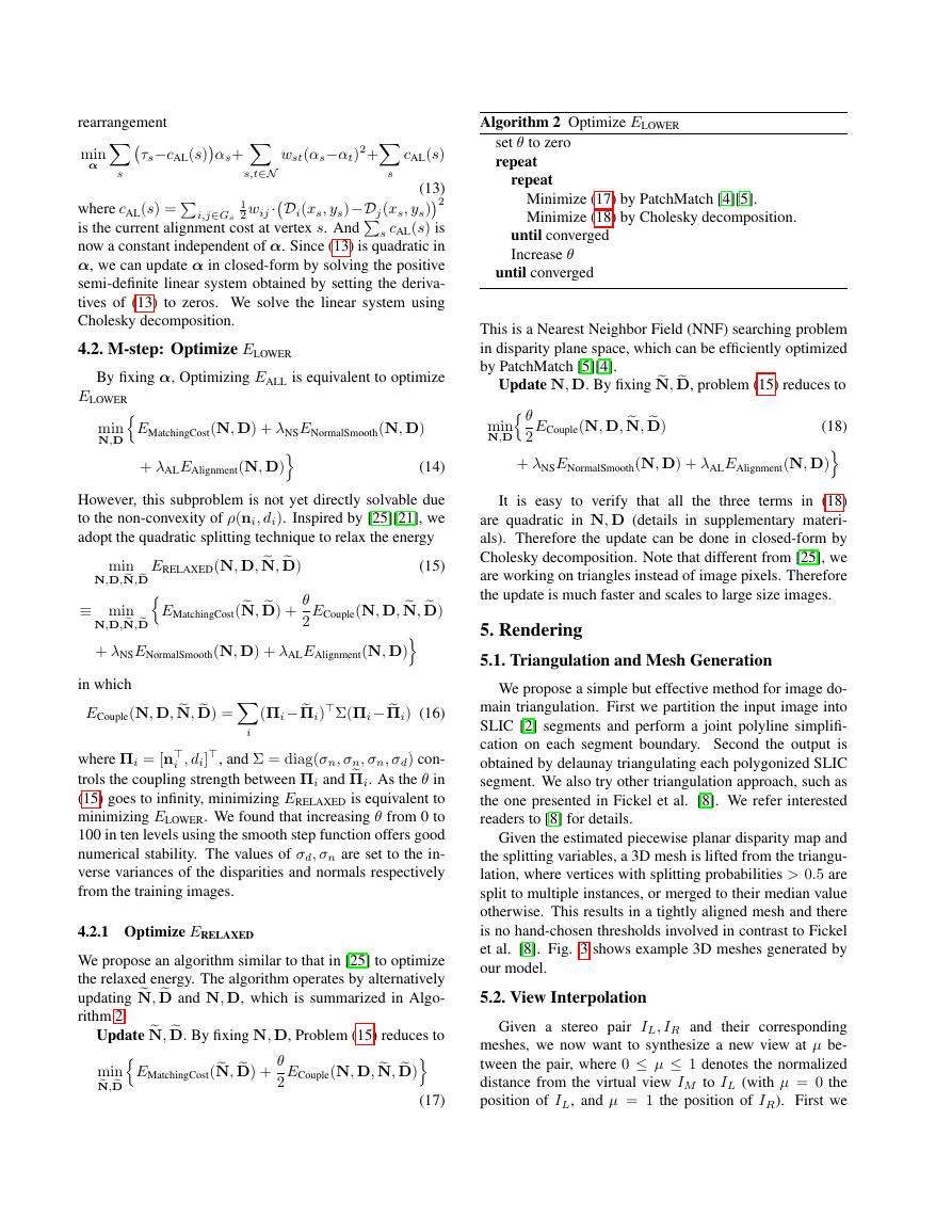This results in a tightly aligned mesh and there is no hand-chosen thresholds involved in contrast to Fickel et al. [8]. Fig. 3 shows example 3D meshes generated by our model. 5.2. View Interpolation Given a stereo pair IL, IR and their corresponding meshes, we now want to synthesize a new view at µ be- tween the pair, where 0 ≤ µ ≤ 1 denotes the normalized distance from the virtual view IM to IL (with µ = 0 the position of IL, and µ = 1 the position of IR). First we

Figure 3. 2D image triangulations and 3D meshes from Middlebury 2.0 generated by our approach. Blue dots in the ﬁrst row represent triangle vertices with splitting probabilities greater than 0.5. Test cases from left to right are (Baby1, Bowling2, Midd1, Plastic, Rocks1) respectively. Results on Baby1,Bowling2 uses our proposed triangulation method, results on Midd1, Plastic, Rocks1 use the one in [8]. 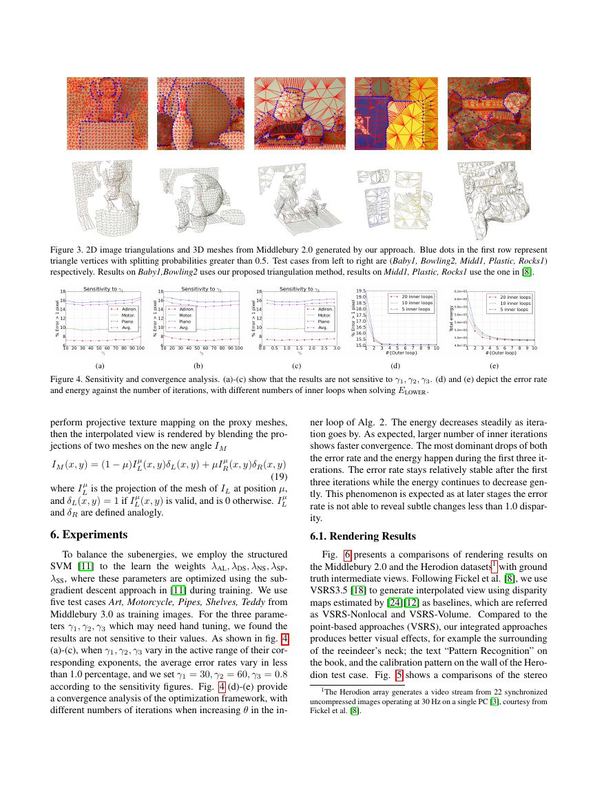(a) (b) (c) (d) (e) Figure 4. Sensitivity and convergence analysis. (a)-(c) show that the results are not sensitive to γ1, γ2, γ3. (d) and (e) depict the error rate and energy against the number of iterations, with different numbers of inner loops when solving ELOWER. perform projective texture mapping on the proxy meshes, then the interpolated view is rendered by blending the pro- jections of two meshes on the new angle IM IM (x, y) = (1 − µ)I µ L(x, y)δL(x, y) + µI µ R(x, y)δR(x, y) (19) L is the projection of the mesh of IL at position µ, L(x, y) is valid, and is 0 otherwise. I µ where I µ and δL(x, y) = 1 if I µ and δR are deﬁned analogly. 6. Experiments L To balance the subenergies, we employ the structured SVM [11] to the learn the weights λAL, λDS, λNS, λSP, λSS, where these parameters are optimized using the sub- gradient descent approach in [11] during training. We use ﬁve test cases Art, Motorcycle, Pipes, Shelves, Teddy from Middlebury 3.0 as training images. For the three parame- ters γ1, γ2, γ3 which may need hand tuning, we found the results are not sensitive to their values. As shown in ﬁg. 4 (a)-(c), when γ1, γ2, γ3 vary in the active range of their cor- responding exponents, the average error rates vary in less than 1.0 percentage, and we set γ1 = 30, γ2 = 60, γ3 = 0.8 according to the sensitivity ﬁgures. Fig. 4 (d)-(e) provide a convergence analysis of the optimization framework, with different numbers of iterations when increasing θ in the in- ner loop of Alg. 2. The energy decreases steadily as itera- tion goes by. As expected, larger number of inner iterations shows faster convergence. The most dominant drops of both the error rate and the energy happen during the ﬁrst three it- erations. The error rate stays relatively stable after the ﬁrst three iterations while the energy continues to decrease gen- tly. This phenomenon is expected as at later stages the error rate is not able to reveal subtle changes less than 1.0 dispar- ity. 6.1. 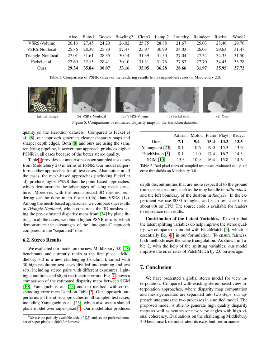Rendering Results Fig. 6 presents a comparisons of rendering results on the Middlebury 2.0 and the Herodion datasets1 with ground truth intermediate views. Following Fickel et al. [8], we use VSRS3.5 [18] to generate interpolated view using disparity maps estimated by [24][12] as baselines, which are referred as VSRS-Nonlocal and VSRS-Volume. Compared to the point-based approaches (VSRS), our integrated approaches produces better visual effects, for example the surrounding of the reeindeer’s neck; the text “Pattern Recognition” on the book, and the calibration pattern on the wall of the Hero- dion test case. Fig. 5 shows a comparisons of the stereo 1The Herodion array generates a video stream from 22 synchronized uncompressed images operating at 30 Hz on a single PC [3], courtesy from Fickel et al. [8].

VSRS-Volume VSRS-Nonlocal Triangle-Nonlocal Fickel et al. Ours 27.45 28.39 31.61 32.15 35.84 Aloe Baby1 Books Bowling2 Cloth3 Lamp.2 Laundry Reindeer Rocks1 Wood2 29.76 26.13 31.47 25.86 31.50 27.01 27.69 33.28 37.72 29.34 24.20 25.83 28.35 28.41 30.07 26.02 27.47 30.14 30.10 33.16 21.67 24.03 27.04 27.82 28.66 25.03 26.03 27.34 27.70 31.97 28.46 29.63 34.35 34.45 35.95 25.75 25.97 31.39 31.31 35.05 28.88 30.99 31.50 31.76 36.28 Table 1. Comparison of PSNR values of the rendering results from sampled test cases on Middlebury 2.0. (a) Left image (b) VSRS-Nonlocal (c) VSRS-Volume (d) Fickel et al. (e) Ours Figure 5. Comparisons of estimated disparity maps on the Herodion datasets. quality on the Herodion datasets. Compared to Fickel et al. [8], our approach generates cleaner disparity maps and sharper depth edges. Both [8] and ours are using the same rendering pipeline, however, our approach produces higher PSNR in all cases because of the better stereo quality. Table 1 provides a comparisons on ten sampled test cases from Middlebury 2.0 in terms of PSNR. Our model outper- forms other approaches for all test cases. Also notice in all the cases, the mesh-based approaches (including Fickel et al), produce higher PSNR than the point-based approaches, which demonstrates the advantages of using mesh struc- ture. Moreover, with the reconstructed 3D meshes, ren- dering can be done much faster (0.1s) than VSRS (1s). Among the mesh-based approaches, we compare our results to Triangle-Nonlocal, which constructs the 3D meshes us- ing the pre-estimated disparity maps from [24] by plane ﬁt- ting. In all the cases, we obtain higher PSNR results, which demonstrates the advantages of the “integrated” approach compared to the “separated” one. 6.2. Stereo Results We evaluated our model on the new Middlebury 3.0 [13] benchmark and currently ranks at the ﬁrst place. 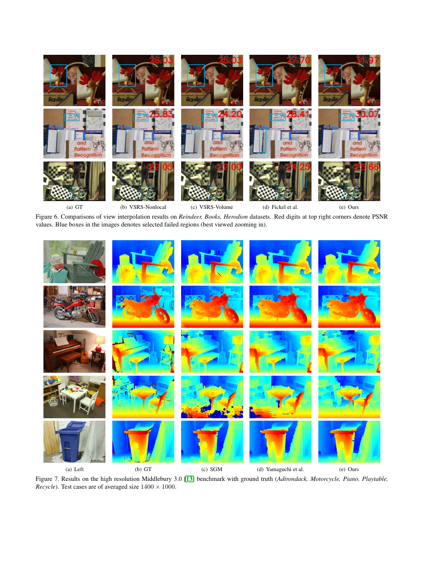Mid- dlebury 3.0 is a new challenging benchmark suited with 30 high resolution test cases divided into training and test sets, including stereo pairs with different exposures, light- ing conditions and slight rectiﬁcation errors. Fig. 7 shows a comparison of the estimated disparity maps between SGM [10], Yamaguchi et al. [23] and our method, with corre- sponding error rates listed on Table 2. Our approach out- performs all the other approaches in all sampled test cases, including Yamaguchi et al. [23], which also uses a slanted plane model over super-pixels2. Our model also produces 2We use the publicly available code of [23] and set the preferred num- ber of super-pixels to 8000 for fairness. Ours Yamaguchi [23] PatchMatch [5] SGM [10] Adiron. Motor. Piano Playt. Recyc. 13.5 13.6 14.3 14.6 15.4 19.0 17.4 16.4 13.3 15.3 16.2 15.8 9.4 10.6 11.0 10.9 7.1 8.1 8.1 15.3 Table 2. Bad pixel rates of sampled test cases evaluated at 1-pixel error thresholds on Middebury 3.0. depth discontinuities that are more respectful to the ground truth scene structure, such as the mug handle in Adirondack, and the left boundary of the dustbin in Recycle. In the ex- periment we use 8000 triangles, and each test case takes about 60s on CPU. The source code is available for readers to reproduce our results. Contribution of the Latent Variables. To verify that the latent splitting variables do help improve the stereo qual- ity, we compare our model with PatchMatch [5], which is essentially Eq. (1) in our formulation. To ensure fairness, both methods uses the same triangulation. As shown in Ta- ble 2, with the help of the splitting variables, our model improve the error rates of PatchMatch by 2.0 on average. 7. Conclusion We have presented a global stereo model for view in- terpolation. Compared with existing stereo-based view in- terpolation approaches, where disparity map computation and mesh generation are separated into two steps, our ap- proach integrates the two processes in a uniﬁed model. The proposed model is able to generate high quality disparity maps as well as synthesize new view angles with high vi- sual coherency. Evaluations on the challenging Middlebury 3.0 benchmark demonstrated its excellent performance.

(a) GT (b) VSRS-Nonlocal (c) VSRS-Volume (d) Fickel et al. (e) Ours Figure 6. Comparisons of view interpolation results on Reindeer, Books, Herodion datasets. Red digits at top right corners denote PSNR values. Blue boxes in the images denotes selected failed regions (best viewed zooming in). (a) Left (b) GT (c) SGM (d) Yamaguchi et al. (e) Ours Figure 7. Results on the high resolution Middlebury 3.0 [13] benchmark with ground truth (Adirondack, Motorcycle, Piano, Playtable, Recycle). Test cases are of averaged size 1400 × 1000.

分享到：

赞收藏

资料库

基于图像分割的立体匹配.pdf

相关推荐

开发技术

热门标签

最新资料