An Introduction to the Kalman Filter Greg Welch 1 and Gary Bishop 2 TR 95-041Department of Computer ScienceUniversity of North Carolina at Chapel HillChapel Hill, NC 27599-3175Updated: Monday, July 24, 2006 Abstract In 1960, R.E. Kalman published his famous paper describing a recursive solution to the discrete-data linear filtering problem. Since that time, due in large part to ad-vances in digital computing, the Kalman filter has been the subject of extensive re-search and application, particularly in the area of autonomous or assisted navigation.The Kalman filter is a set of mathematical equations that provides an efficient com-putational (recursive) means to estimate the state of a process, in a way that mini-mizes the mean of the squared error. The filter is very powerful in several aspects: it supports estimations of past, present, and even future states, and it can do so even when the precise nature of the modeled system is unknown.The purpose of this paper is to provide a practical introduction to the discrete Kal-man filter. This introduction includes a description and some discussion of the basic discrete Kalman filter, a derivation, description and some discussion of the extend-ed Kalman filter, and a relatively simple (tangible) example with real numbers & results. 1. welch@cs.unc.edu, http://www.cs.unc.edu/~welch 2. gb@cs.unc.edu, http://www.cs.unc.edu/~gb�
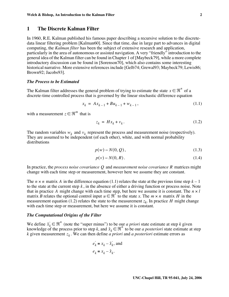
Welch & Bishop, An Introduction to the Kalman Filter2UNC-Chapel Hill, TR 95-041, July 24, 2006 1The Discrete Kalman Filter In 1960, R.E. Kalman published his famous paper describing a recursive solution to the discrete-data linear filtering problem [Kalman60]. Since that time, due in large part to advances in digital computing, the Kalman filter has been the subject of extensive research and application, particularly in the area of autonomous or assisted navigation. A very “friendly” introduction to the general idea of the Kalman filter can be found in Chapter 1 of [Maybeck79], while a more complete introductory discussion can be found in [Sorenson70], which also contains some interesting historical narrative. More extensive references include [Gelb74; Grewal93; Maybeck79; Lewis86; Brown92; Jacobs93]. The Process to be Estimated The Kalman filter addresses the general problem of trying to estimate the state of a discrete-time controlled process that is governed by the linear stochastic difference equation,(1.1)with a measurement that is.(1.2)The random variables and represent the process and measurement noise (respectively). They are assumed to be independent (of each other), white, and with normal probability distributions,(1.3).(1.4)In practice, the process noise covariance and measurement noise covariance matrices might change with each time step or measurement, however here we assume they are constant.The matrix in the difference equation (1.1) relates the state at the previous time step to the state at the current step , in the absence of either a driving function or process noise. Note that in practice might change with each time step, but here we assume it is constant. The matrix B relates the optional control input to the state x . The matrix in the measurement equation (1.2) relates the state to the measurement z k . In practice might change with each time step or measurement, but here we assume it is constant. The Computational Origins of the Filter We define (note the “super minus”) to be our a priori state estimate at step k given knowledge of the process prior to step k , and to be our a posteriori state estimate at step k given measurement . We can then define a priori and a posteriori estimate errors asxℜn∈xkAxk1–Buk1–wk1–++=zℜm∈zkHxkvk+=wkvkpw()N0Q,()∼pv()N0R,()∼QRnn×Ak1–kAnl×uℜl∈mn×HHxˆk-ℜn∈xˆkℜn∈zkek-xkxˆk-, and–≡ekxkxˆk.–≡�
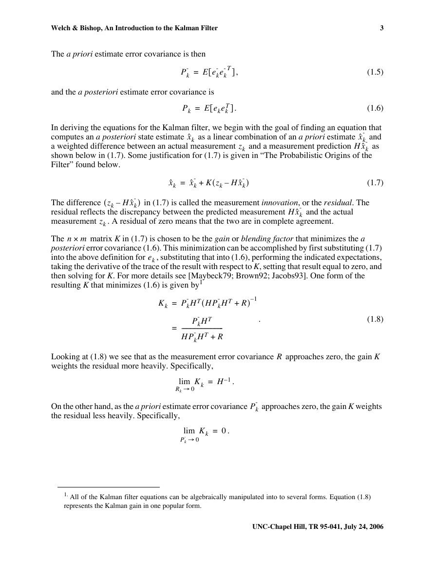
Welch & Bishop, An Introduction to the Kalman Filter3UNC-Chapel Hill, TR 95-041, July 24, 2006 The a priori estimate error covariance is then,(1.5)and the a posteriori estimate error covariance is.(1.6)In deriving the equations for the Kalman filter, we begin with the goal of finding an equation that computes an a posteriori state estimate as a linear combination of an a priori estimate and a weighted difference between an actual measurement and a measurement prediction as shown below in (1.7). Some justification for (1.7) is given in “The Probabilistic Origins of the Filter” found below.(1.7)The difference in (1.7) is called the measurement innovation , or the residual . The residual reflects the discrepancy between the predicted measurement and the actual measurement . A residual of zero means that the two are in complete agreement. The matrix K in (1.7) is chosen to be the gain or blending factor that minimizes the a posteriori error covariance (1.6). This minimization can be accomplished by first substituting (1.7) into the above definition for , substituting that into (1.6), performing the indicated expectations, taking the derivative of the trace of the result with respect to K , setting that result equal to zero, and then solving for K . For more details see [Maybeck79; Brown92; Jacobs93]. One form of the resulting K that minimizes (1.6) is given by 1 .(1.8)Looking at (1.8) we see that as the measurement error covariance approaches zero, the gain K weights the residual more heavily. Specifically,.On the other hand, as the a priori estimate error covariance approaches zero, the gain K weights the residual less heavily. Specifically,. 1. All of the Kalman filter equations can be algebraically manipulated into to several forms. Equation (1.8)represents the Kalman gain in one popular form.Pk-Eek-ek-T[]=PkEekekT[]=xˆkxˆk-zkHxˆk-xˆkxˆk-KzkHxˆk-–()+=zkHxˆk-–()Hxˆk-zknm×ekKkPk-HTHPk-HTR+()1–=Pk-HTHPk-HTR+-----------------------------=RKkRk0→limH1–=Pk-KkPk-0→lim0=�
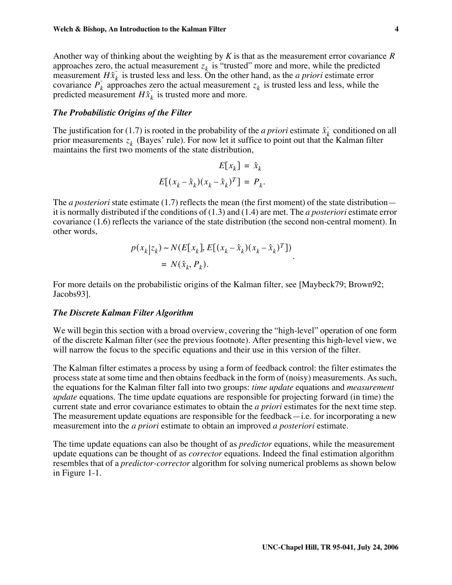
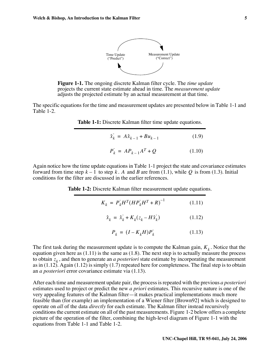
Welch & Bishop, An Introduction to the Kalman Filter4UNC-Chapel Hill, TR 95-041, July 24, 2006Another way of thinking about the weighting by K is that as the measurement error covariance approaches zero, the actual measurement is “trusted” more and more, while the predicted measurement is trusted less and less. On the other hand, as the a priori estimate error covariance approaches zero the actual measurement is trusted less and less, while the predicted measurement is trusted more and more.The Probabilistic Origins of the FilterThe justification for (1.7) is rooted in the probability of the a priori estimate conditioned on all prior measurements (Bayes’ rule). For now let it suffice to point out that the Kalman filter maintains the first two moments of the state distribution,The a posteriori state estimate (1.7) reflects the mean (the first moment) of the state distribution— it is normally distributed if the conditions of (1.3) and (1.4) are met. The a posteriori estimate error covariance (1.6) reflects the variance of the state distribution (the second non-central moment). In other words,.For more details on the probabilistic origins of the Kalman filter, see [Maybeck79; Brown92; Jacobs93].The Discrete Kalman Filter AlgorithmWe will begin this section with a broad overview, covering the “high-level” operation of one form of the discrete Kalman filter (see the previous footnote). After presenting this high-level view, we will narrow the focus to the specific equations and their use in this version of the filter.The Kalman filter estimates a process by using a form of feedback control: the filter estimates the process state at some time and then obtains feedback in the form of (noisy) measurements. As such, the equations for the Kalman filter fall into two groups: time update equations and measurement update equations. The time update equations are responsible for projecting forward (in time) the current state and error covariance estimates to obtain the a priori estimates for the next time step. The measurement update equations are responsible for the feedback—i.e. for incorporating a new measurement into the a priori estimate to obtain an improved a posteriori estimate.The time update equations can also be thought of as predictor equations, while the measurement update equations can be thought of as corrector equations. Indeed the final estimation algorithm resembles that of a predictor-corrector algorithm for solving numerical problems as shown below in Figure 1-1.RzkHxˆk-Pk-zkHxˆk-xˆk-zkExk[]xˆk=Exkxˆk–()xkxˆk–()T[]Pk.=pxkzk()NExk[]Exkxˆk–()xkxˆk–()T[],()∼NxˆkPk,().=�
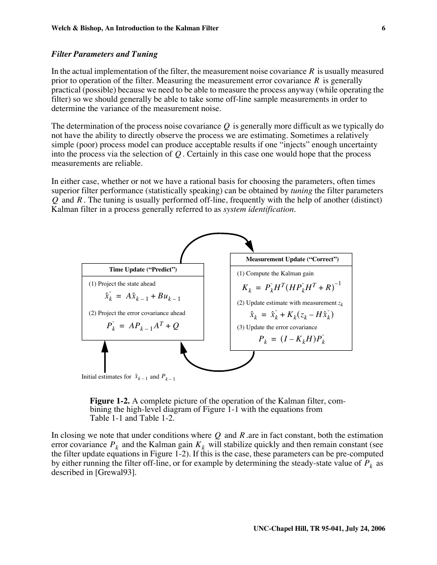
Welch & Bishop, An Introduction to the Kalman Filter5UNC-Chapel Hill, TR 95-041, July 24, 2006Figure 1-1. The ongoing discrete Kalman filter cycle. The time update projects the current state estimate ahead in time. The measurement update adjusts the projected estimate by an actual measurement at that time.The specific equations for the time and measurement updates are presented below in Table 1-1 and Table 1-2.Again notice how the time update equations in Table 1-1 project the state and covariance estimates forward from time step to step . and B are from (1.1), while is from (1.3). Initial conditions for the filter are discussed in the earlier references.The first task during the measurement update is to compute the Kalman gain, . Notice that the equation given here as (1.11) is the same as (1.8). The next step is to actually measure the process to obtain , and then to generate an a posteriori state estimate by incorporating the measurement as in (1.12). Again (1.12) is simply (1.7) repeated here for completeness. The final step is to obtain an a posteriori error covariance estimate via (1.13).After each time and measurement update pair, the process is repeated with the previous a posteriori estimates used to project or predict the new a priori estimates. This recursive nature is one of the very appealing features of the Kalman filter—it makes practical implementations much more feasible than (for example) an implementation of a Wiener filter [Brown92] which is designed to operate on all of the data directly for each estimate. The Kalman filter instead recursively conditions the current estimate on all of the past measurements. Figure 1-2 below offers a complete picture of the operation of the filter, combining the high-level diagram of Figure 1-1 with the equations from Table 1-1 and Table 1-2.Table 1-1: Discrete Kalman filter time update equations.(1.9)(1.10)Table 1-2: Discrete Kalman filter measurement update equations.(1.11)(1.12)(1.13)Time Update(“Predict”)Measurement Update(“Correct”)xˆk-Axˆk1–Buk1–+=Pk-APk1–ATQ+=k1–kAQKkPk-HTHPk-HTR+()1–=xˆkxˆk-KkzkHxˆk-–()+=PkIKkH–()Pk-=Kkzk�
Welch & Bishop, An Introduction to the Kalman Filter6UNC-Chapel Hill, TR 95-041, July 24, 2006Filter Parameters and TuningIn the actual implementation of the filter, the measurement noise covariance is usually measured prior to operation of the filter. Measuring the measurement error covariance is generally practical (possible) because we need to be able to measure the process anyway (while operating the filter) so we should generally be able to take some off-line sample measurements in order to determine the variance of the measurement noise.The determination of the process noise covariance is generally more difficult as we typically do not have the ability to directly observe the process we are estimating. Sometimes a relatively simple (poor) process model can produce acceptable results if one “injects” enough uncertainty into the process via the selection of . Certainly in this case one would hope that the process measurements are reliable.In either case, whether or not we have a rational basis for choosing the parameters, often times superior filter performance (statistically speaking) can be obtained by tuning the filter parameters and . The tuning is usually performed off-line, frequently with the help of another (distinct) Kalman filter in a process generally referred to as system identification.Figure 1-2. A complete picture of the operation of the Kalman filter, com-bining the high-level diagram of Figure 1-1 with the equations from Table 1-1 and Table 1-2.In closing we note that under conditions where and .are in fact constant, both the estimation error covariance and the Kalman gain will stabilize quickly and then remain constant (see the filter update equations in Figure 1-2). If this is the case, these parameters can be pre-computed by either running the filter off-line, or for example by determining the steady-state value of as described in [Grewal93].RRQQQRKkPk-HTHPk-HTR+()1–=(1) Compute the Kalman gainxˆk1–Initial estimates for andPk1–xˆkxˆk-KkzkHxˆk-–()+=(2) Update estimate with measurement zk(3) Update the error covariancePkIKkH–()Pk-=Measurement Update (“Correct”)(1) Project the state ahead(2) Project the error covariance aheadTime Update (“Predict”)xˆk-Axˆk1–Buk1–+=Pk-APk1–ATQ+=QRPkKkPk�
Welch & Bishop, An Introduction to the Kalman Filter7UNC-Chapel Hill, TR 95-041, July 24, 2006It is frequently the case however that the measurement error (in particular) does not remain constant. For example, when sighting beacons in our optoelectronic tracker ceiling panels, the noise in measurements of nearby beacons will be smaller than that in far-away beacons. Also, the process noise is sometimes changed dynamically during filter operation—becoming —in order to adjust to different dynamics. For example, in the case of tracking the head of a user of a 3D virtual environment we might reduce the magnitude of if the user seems to be moving slowly, and increase the magnitude if the dynamics start changing rapidly. In such cases might be chosen to account for both uncertainty about the user’s intentions and uncertainty in the model.2The Extended Kalman Filter (EKF)The Process to be EstimatedAs described above in section 1, the Kalman filter addresses the general problem of trying to estimate the state of a discrete-time controlled process that is governed by a linear stochastic difference equation. But what happens if the process to be estimated and (or) the measurement relationship to the process is non-linear? Some of the most interesting and successful applications of Kalman filtering have been such situations. A Kalman filter that linearizes about the current mean and covariance is referred to as an extended Kalman filter or EKF.In something akin to a Taylor series, we can linearize the estimation around the current estimate using the partial derivatives of the process and measurement functions to compute estimates even in the face of non-linear relationships. To do so, we must begin by modifying some of the material presented in section 1. Let us assume that our process again has a state vector , but that the process is now governed by the non-linear stochastic difference equation,(2.1)with a measurement that is,(2.2)where the random variables and again represent the process and measurement noise as in (1.3) and (1.4). In this case the non-linear function in the difference equation (2.1) relates the state at the previous time step to the state at the current time step . It includes as parameters any driving function and the zero-mean process noise wk. The non-linear function in the measurement equation (2.2) relates the state to the measurement .In practice of course one does not know the individual values of the noise and at each time step. However, one can approximate the state and measurement vector without them as(2.3)and,(2.4)where is some a posteriori estimate of the state (from a previous time step k).QQkQkQkxℜn∈xℜn∈xkfxk1–uk1–wk1–,,()=zℜm∈zkhxkvk,()=wkvkfk1–kuk1–hxkzkwkvkx˜kfxˆk1–uk1–0,,()=z˜khx˜k0,()=xˆk�
Welch & Bishop, An Introduction to the Kalman Filter8UNC-Chapel Hill, TR 95-041, July 24, 2006It is important to note that a fundamental flaw of the EKF is that the distributions (or densities in the continuous case) of the various random variables are no longer normal after undergoing their respective nonlinear transformations. The EKF is simply an ad hoc state estimator that only approximates the optimality of Bayes’ rule by linearization. Some interesting work has been done by Julier et al. in developing a variation to the EKF, using methods that preserve the normal distributions throughout the non-linear transformations [Julier96].The Computational Origins of the FilterTo estimate a process with non-linear difference and measurement relationships, we begin by writing new governing equations that linearize an estimate about (2.3) and (2.4),,(2.5).(2.6)where• and are the actual state and measurement vectors,• and are the approximate state and measurement vectors from (2.3) and (2.4),• is an a posteriori estimate of the state at step k,•the random variables and represent the process and measurement noise as in (1.3) and (1.4). •A is the Jacobian matrix of partial derivatives of with respect to x, that is,•W is the Jacobian matrix of partial derivatives of with respect to w,,•H is the Jacobian matrix of partial derivatives of with respect to x,,•V is the Jacobian matrix of partial derivatives of with respect to v,.Note that for simplicity in the notation we do not use the time step subscript with the Jacobians , , , and , even though they are in fact different at each time step.xkx˜kAxk1–xˆk1––()Wwk1–++≈zkz˜kHxkx˜k–()Vvk++≈xkzkx˜kz˜kxˆkwkvkfAij,[]xj[]∂∂fi[]xˆk1–uk1–0,,()=fWij,[]wj[]∂∂fi[]xˆk1–uk1–0,,()=hHij,[]xj[]∂∂hi[]x˜k0,()=hVij,[]vj[]∂∂hi[]x˜k0,()=kAWHV�


 2023年江西萍乡中考道德与法治真题及答案.doc
 2012年重庆南川中考生物真题及答案.doc
 2013年江西师范大学地理学综合及文艺理论基础考研真题.doc
 2020年四川甘孜小升初语文真题及答案I卷.doc
 2020年注册岩土工程师专业基础考试真题及答案.doc
 2023-2024学年福建省厦门市九年级上学期数学月考试题及答案.doc
 2021-2022学年辽宁省沈阳市大东区九年级上学期语文期末试题及答案.doc
 2022-2023学年北京东城区初三第一学期物理期末试卷及答案.doc
 2018上半年江西教师资格初中地理学科知识与教学能力真题及答案.doc
 2012年河北国家公务员申论考试真题及答案-省级.doc
 2020-2021学年江苏省扬州市江都区邵樊片九年级上学期数学第一次质量检测试题及答案.doc
 2022下半年黑龙江教师资格证中学综合素质真题及答案.doc